Calculation of Statistical Strength

Static calculation of the structure (or other analyzed the strength test is performed under the assumption that the boundary conditions and the applied loads are constant or slow to change over time; at the same time mechanical vibrations or transient thermal processes missing. Within the framework of static calculation, the following tasks can be solved:

elasticity (in linear formulation);
plasticity (physical nonlinearity);
analysis finite deformations (geometric nonlinearity);
thermal conductivity;
multistep loads.

When solving elasticity problems in a linear formulation , assumptions apply, that the calculated construction returns to the original undeformed the condition after unloading, deformation and displacement in the model are as a rule, small deformations are considered to be about 10% of the characteristic size), stresses do not reach the yield point. When solving problems of plasticity and analysis of finite deformations, the effects arising are taken into account with large deformations of the structure.

The fields of static strength calculation output are configured from the Command Panel by selecting (Mode - Calculation Settings, Calculation Settings - Static, Static - General) (it is assumed that the user has already built a finite element model analyzed object, set boundary conditions and loads).

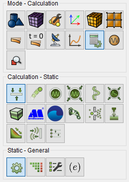
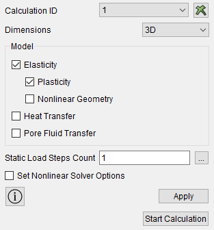
Fig. 1 - Command panel, general settings for static calculation

In the drop-down list Dimensions choose the dimension of the problem to be solved: 3D (three-dimensional) or 2D (flat).

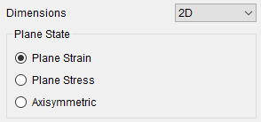
In the case of 2D, you must optionally select Plane state: Plane strain, Plane stress or Axisymmetric. The first two types of problems are flat in the usual sense, while the axisymmetric problem, although it has a two-dimensional setting, should be taken as three-dimensional. For more information on axisymmetric task setting, see the end of the section.
If necessary, you can use spectral element method; to do this, check the appropriate boxes.
In the checkbox group Model select the checkbox corresponding to the features of the model used solutions:

Elasticity;
Plasticity;
Nonlinear geometry;
Heat transfer;
Pore Fluid Transfer.

At the same time, combinations of models (checkboxes) are also possible, for example:

Elastic-plasticity (checkboxes Elasticity and Plasticity);
Thermoelasticity (check boxes Elasticity and Heat transfer).

To solve a nonlinear problem check the box To set the settings of the nonlinear solver. The corresponding input windows will open:

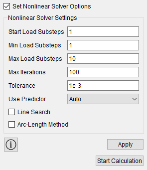
Fig. 2 - Command Panel, settings of the nonlinear solver

You can leave the default values in them, or specify the required by the user.

Notes: Load in a non-linear the task is applied as a sequence of steps. The system of nonlinear The equations are solved using Newton's iterative method. When reaching the specified accuracy of the solution or the maximum number of iterations of the process the solution is being completed.

Further settings are made as follows:

On the Command Bar among the settings for static calculation, select the icon ( Static - Solver).
Perform the necessary solver settings for using direct or iterative solution methods.
Configure the output fields of the results calculation (Static - Output Fields):

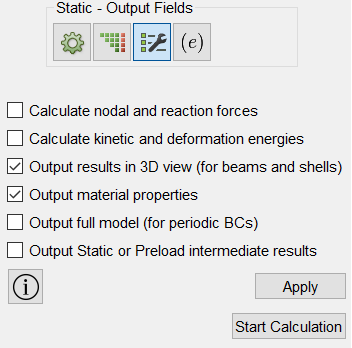
Fig. 3 - Panel commands,settings of output fields for static calculation

The necessary information on this setting is given in the subsection Customization output fields during static calculation.

Click Apply.

Click Start Calculation.

In a pop-up window select a folder to save the result and enter the file name.

In the case of a successful calculation, the console displays the message: Calculation finished successfully at "date" "time".

To display the calculation results, you can use icon (Open the results of the last calculation). Clicking on this icon starts the Fidesys postprocessor: program FidesysViewer. A description of the operation of this program is given in a separate manual.

Let's give more detailed information about the Axisymmetric task setting (one of the variants of the Task type). In the case of this statement, it is assumed that the body is three-dimensional and radially symmetrical about the Y axis. Moreover, all loads (and boundary and initial conditions) are also applied symmetrically. A solution to this problem is possible in 2D, where a two-dimensional surface is considered, the rotation of which about the Y axis by 360 degrees constitutes the original body.

Thus, in the case of choosing the Axisymmetric type of the problem, you should build a figure on the OXY plane, x≥0, perceiving it as the body of rotation of this surface around the Y axis. Permissible boundary conditions in this setting: restriction of movements, velocities; pressure; distributed force; set temperature; convection; pore pressure.

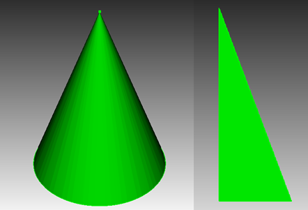
Fig. 4 - The body of rotation (the cone on the left) and its two-dimensional representation (the triangle on the right) in an axisymmetric formulation

It follows from the axial symmetry condition that the points of a two-dimensional surface can only move in the radial (X) or axial (Y) direction. Points located on the axis of symmetry (x=0) can only move in the axial (Y) direction. These conditions are met automatically when an Axisymmetric task type is selected.

You can see examples of this calculation here: