Search the documentation
Enter at least 2 characters
Enter at least 2 characters
 |
CAE Fidesys 9.0 Documentation |
S.H. Crandall, N.C. Dahl, An Introduction to the Mechanics of Solids, McGraw-Hill Book Co., Inc., New York, NY, 1959, pg. 389, ex. 8.9.
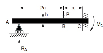
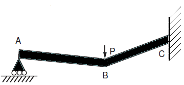
The problem of static load of a square section beam is being solved. The picture represents a geometric model of the problem: a = 50 In, beam section 1 x 1 in. The boundary conditions are presented in the picture; the force applied at the point B is Fy = -1000 lb. The material parameters are E = 30e6 psi, ν = 0.3.
Test pass criterion is the following: reaction force RA at the point A (0,0,0) is 148.15 lb, reaction moment at the point C is 27778 in-lb within 1.5%.
1. Create a straight line 100 in length (segment AB).
On the command bar, select the module for constructing geometry (Mode — Geometry, Entity — Curve, Action — Create).
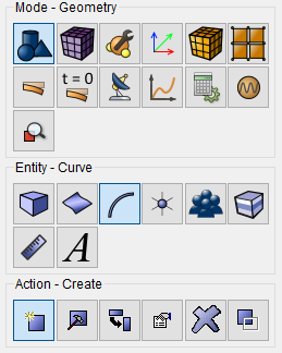
Select Line in the list of geometric elements. Create it using Location and Direction.
Set the following parameters:
Location: 0 0 0 (line origin);
Direction: 1 0 0 (along Х axis);
Length: 100.
Click Apply.
2. Create a straight line 50 in length (segment BC).
On the command bar, select the module for constructing geometry (Mode — Geometry, Entity — Curve, Action — Create).
Select Line in the list of geometric elements. Create it using Location and Direction.
Set the following parameters:
Location: 100 0 0 (line origin);
Direction: 1 0 0 (along Х axis);
Length: 50.
Click Apply.
As a result, in left side of the Model Tree there are two free curves having no common vertices.
3. Unite two vertices.
On the command bar, select the module for constructing geometry (Mode — Geometry, Entity — Vertex, Action — Merge).
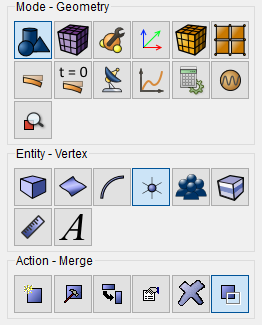
Set the following parameters:
Vertex ID(s): 2 3 (using space after each of them).
Click Apply.
1. On the command bar, select the mesh module (Mode — Mesh, Entity — Curve, Action — Mesh).
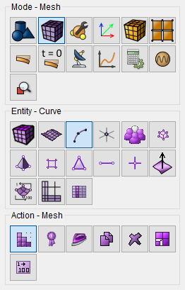
Specify the parameters of mesh refinement:
Select Curves: all;
Select the way of meshing: Equal;
Select the meshing parameters: Interval;
Interval: 1.
Click Apply Size.
Click Mesh.
1. Fix the point C at all directions.
On the command panel, select the boundary conditions module (Mode — Boundary Conditions, Entity — Displacement, Action — Create).
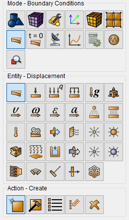
Set the following parameters:
Entity List: Vertex;
Entity ID(s): 4;
Degrees of Freedom: Fix All.
Click Apply.
2. Fix the point A at the Y and Z displacement.
On the command panel, select the boundary conditions module (Mode — Boundary Conditions, Entity — Displacement, Action — Create).
Set the following parameters:
Entity List: Vertex;
Entity ID(s): 1;
Degrees of Freedom: Y, Z.
Click Apply.
3. Apply force at the point B.
On the command panel, select the boundary conditions module (Mode — Boundary Conditions, Entity — Force, Action — Create).
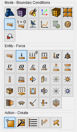
Set the following parameters:
Entity List: Vertex;
Entity ID(s): 2;
Force: 1000;
Direction 0 -1 0.
Click Apply.
1. Create the material.
In the command bar, select the module for specifying material properties (Mode — Material, Entity — Materials Management).

In the Materials Management window that opens, in the second column, click on the caption Enter the name of the material and write “Material1”.
Click the ENTER key.
In the left column, select Elasticity - Isotropic Material. Select with the mouse the characteristic Young's modulus. Hold down the left mouse button and drag the label to Material Properties. Double-click in the Value field next to Young’s modulus and enter the number 3e+07. Similarly, from the Isotropic Material section add the Poisson ratio 0.
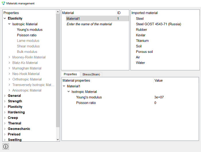
Click Apply.
Close the Materials management window.
2. Create the block of one type of the material.
On the command bar, select the block management module (Mode — Blocks, Entity — Block, Action — Add).

Set the following parameters:
Block ID: 1;
Entity List: Curve;
Entity ID(s): 1 2 (or by the command all).
Click Apply.
3. Set the block parameters.
On the command bar, select the block management module (Mode - Blocks, Entity - Block, Action - Block properties/parameters).

Set the following parameters:
Block ID(s): 1;
Category: Beam;
Material: Material1;
Coordinate System: Global Cartesian;
Order: 1.
Set the beam properties by clicking the button  .
From the profile section drop-down list, select Rectangle.
.
From the profile section drop-down list, select Rectangle.
Specify the following parameters:
Height (H): 1;
Width (B): 1.
Click Apply.
Close the window Set Beam Properties.
Click Apply.
1. Set the type of the problem to be solved.
On the command bar, select the calculation settings module (Mode — Calculation Settings, Calculation Settings — Static, Static — General).
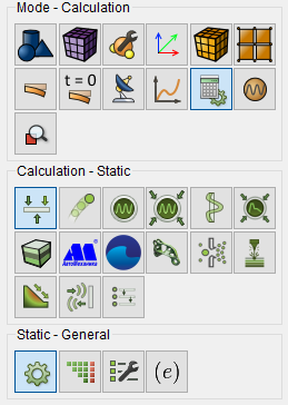
Select:
Dimensions: 3D;
Model: Elasticity.
Click Apply.
2. Set the solver settings.
On the command bar, select the calculation settings module (Mode — Calculation Settings, Calculation settings — Static, Static — Solver).
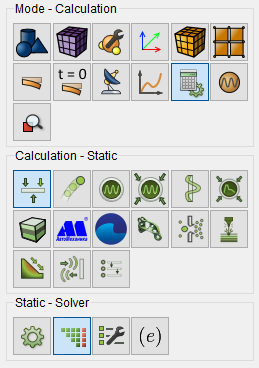
Select the solver method (direct or iterative) and set Convergence Parameters in case of choosing an iterative one. You can also leave all the settings by default.
Click Apply.
3. Set the reaction force calculation.
On the command bar, select the calculation settings module (Mode — Calculation Settings, Calculation settings — Static, Static — Output Fields).
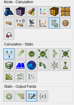
Set the flag Nodal and Reaction Forces.
Set the flag Results in 3D View (for Beams and Shells).
Click Apply.
Click Start Calculation.
Note: Without setting the checkbox Nodal and Reaction Forces, the field is not calculated.
4. In a pop-up window select a folder to save the result and enter the file name.
5. In the case of a successful calculation, the console displays the message: Calculation finished successfully at "date" "time".
1. Open the file with the results. There are three ways to do that.
Click Ctrl+E.
From the main menu, select Calculation. Click Open Results.
Select Results on Command Panel (Mode - Results). Click Open results.

2. Display the Uy component of the displacements field.
In FidesysViewer window set the following parameters on Toolbar:
Representation Mode: Surface;
Representation Field: Displacement;
Representation Component: Y.
The field of displacements distribution along the Y axis wil be displayed on the model.

To automatically apply changes to all filters on the command bar, click
the corresponding Apply changes to parameters automatically button.-
 .
.
3. Check the numerical value of the reaction force at the point A.
Display Component Y of the Reaction Force field.

On the FidesysViewer Main Panel, click Select Points On surface.
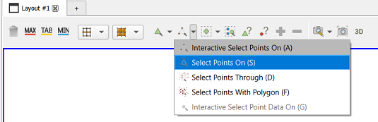
Select the limiting left point (point A) on the geometric model.
To quickly view the information at the fixed point, click pointsInfo on the Main Panel.

In the pop-up window, components of the reaction force at the selected point will be displayed.
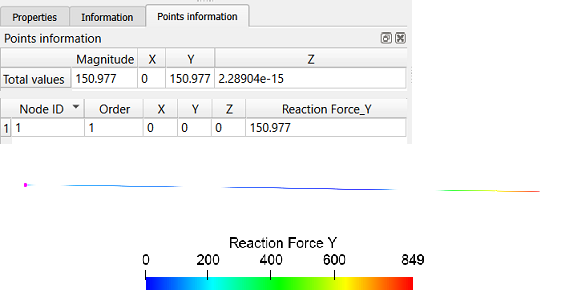
The difference between the resulting value 150.977 and the required 148.15 is less than 1,9%.
Do not close the window Points information.
4. Check the numerical value of reaction moments at the point C.
Display Component Z of the Reaction Moment field.

On the FidesysViewer Main Panel, click Select Points On surface.
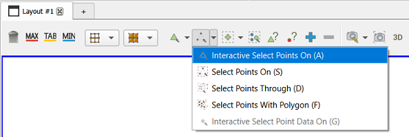
Select the limiting right point C on the geometric model.
In the window Points information components of the reaction moment at the selected point will be displayed.
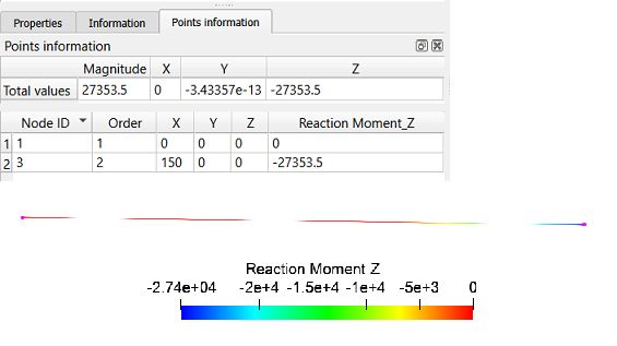
The difference between the resulting value -27353.5 and the required -27778 is less than 1.6%.
5. Open 3D-image of the beam.
To display a 3D view of the beam section, focus on the calculation name
and click the 3D View button on the command bar.  .
.
6. Download numerical data.
Select File → Save Data in the Main Menu or click Ctrl+S. Enter the file name (*.csv format), leave it by default. Click ОК. The saved file is an ordinary table of numerical data, any text editor can open it.
Geometry creating, meshing, setting boundary conditions and materials can be performed using the console interface. Below is a link to the program code that allows you to perform the steps described above manual, you only need to specify the full path and name.