Search the documentation
Enter at least 2 characters
Enter at least 2 characters
 |
CAE Fidesys 9.0 Documentation |
Timoshenko S.P. Voynovskiy-Kriger S. Plates and shells, Nauka, Moscow, - 1966, 636 pages [in Russian]
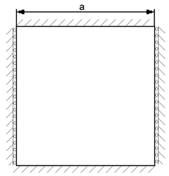
We solve the problem of static load of square shell the two sides of which are clamped and the other two are freely supported.The picture represents a geometric model of the problem: a = 1 m, shell thickness is 0.1 m. The boundary conditions are presented in the picture. The plate is loaded by uniform pressure of 10 kPa.
Test pass criterion is the following: the maximum deflection is 1.19e-6, moments M x = 252 N·m and M y = 332 N·m.
1. Create the square 1 m on side.
On the command bar, select the module for constructing surface geometry (Mode - Geometry, Entity - Surface, Action - Create).
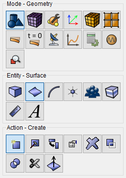
Select Rectangle in the list of geometric elements.
Set the parameters:
Width: 1;
Height: Optional;
ZPlane.
Click Apply.
1. On the command bar, select the surface mesh module (Mode - Mesh, Entity - Surface, Action - Mesh).
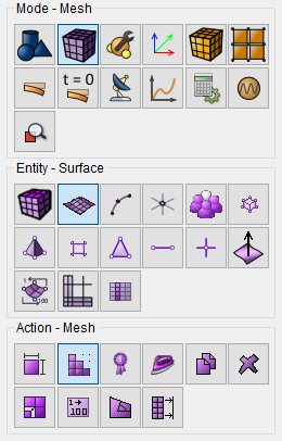
Specify the following parameters:
Select meshing scheme: Polyhedron;
Select Surfaces: 1.
Click Apply Scheme.
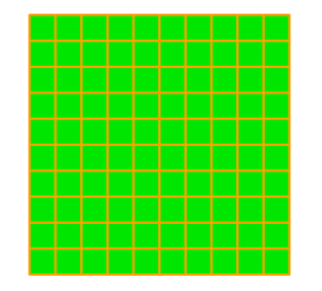
Click Mesh.
1. Fix the two edges rigidly.
On the command panel, select the boundary conditions module (Mode - Boundary Conditions, Entity - Displacement, Action - Create).
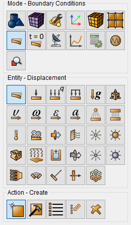
Set the following parameters:
Entity List: Curve;
Entity ID(s): 1 3 (or sequentially click on the top and bottom edges);
Degrees of Freedom: Fix All.
Click Apply.
2. Fix the other two edges at displacements.
On the command panel, select the boundary conditions module (Mode - Boundary Conditions, Entity - Displacement, Action - Create).
Set the following parameters:
Entity List: Curve;
Entity ID(s): 2 4 (or sequentially click on the right and left edges);
Degrees of Freedom: X, Y, Z.
Click Apply.
3. Apply the uniform pressure on the surface.
On the command panel, select the boundary conditions module (Mode - Boundary Conditions, Entity - Pressure, Action - Create).
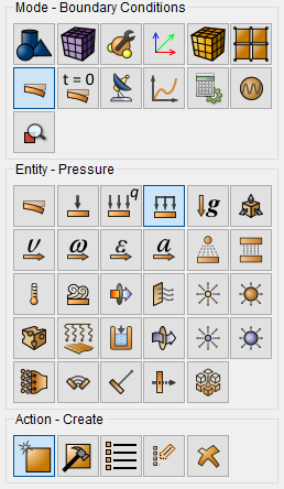
Set the following parameters:
Entity List: Surface;
Entity ID(s): 1;
Value: 1e4.
Click Apply.
1. Create the material.
In the command bar, select the module for specifying material properties (Mode - Material, Entity - Materials Management).

In the Materials Management window that opens, in the second column, click the caption “Enter the name of the material” and write “Material 1”.
Click the ENTER key.
In the left column, select Elasticity - Isotropic Material. Select with the mouse the characteristic Young's modulus. Hold down the left mouse button and drag the label to Material Properties. Double-click in the Value field next to Young's modulus and enter the number 2e+11.Similarly add the Poisson ratio 0.3 from the Isotropic Material section.
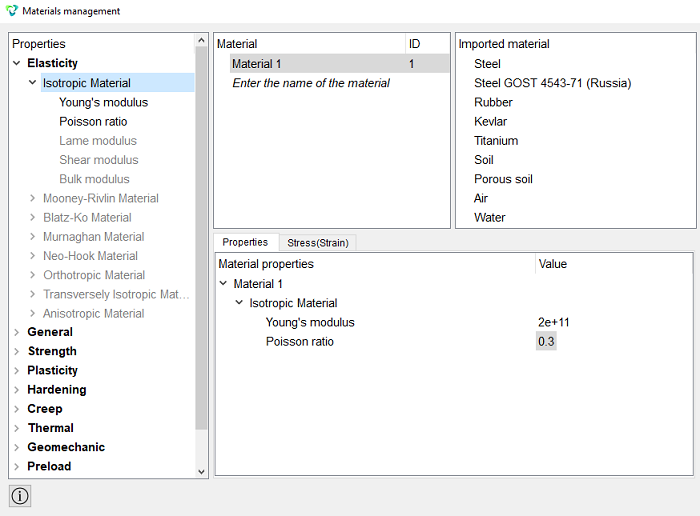
Click Apply.
Close the Materials management window.
2. Create the block of one type of the material.
On the command bar, select the block management module (Mode - Blocks, Entity - Block, Action - Add).

Set the following parameters:
Block ID: 1;
Entity List: Surface;
Entity ID(s): 1 (or by the command all).
Click Apply.
3. Set the block parameters.
On the command bar, select the block management module (Mode - Blocks, Entity - Block, Action - Block properties/parameters).

Set the following parameters:
Block ID(s): 1;
Category: Shell;
Coordinate System: Global Cartesian;
Order: 1.
Set the shell properties by clicking the button  .
.
Set the following parameters:
Material: Material 1;
Thickness: 0.1;
Eccentricity: 0.5.
Click Apply.
Close the window Set Shell Properties.
Click Apply.
1. Set the type of the problem to be solved.
On the command bar, select the calculation settings module (Mode - Calculation Settings, Calculation Settings - Static, Static - General).
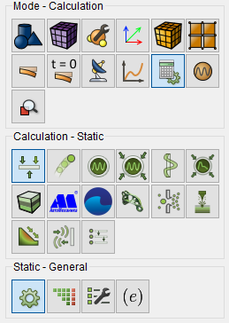
Select:
Dimensions: 3D;
Model: Elasticity.
Click Apply.
2. Set the solver settings.
On the command bar, select the calculation settings module (Mode - Calculation Settings, Calculation settings - Static, Static - Solver).
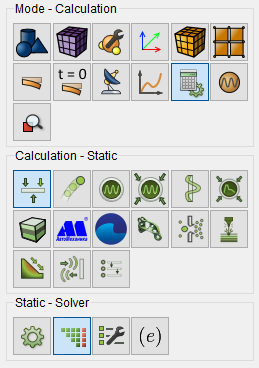
Select the solver method (direct or iterative) and set Convergence Parameters in case of choosing an iterative one. You can also leave all the settings by default.
Click Apply.
3. Set the reaction force calculation
On the command bar, select the calculation settings module (Mode — Calculation Settings, Calculation settings — Static, Static — Output Fields).
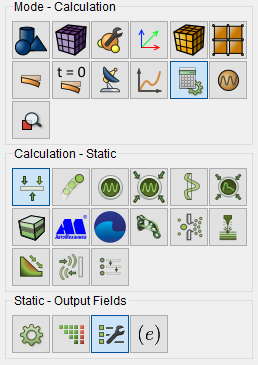
Set the flag Nodal and Reaction Forces.
Set the flag Results in 3D View (for Beams and Shells).
Click Apply.
Click Start Calculation.
Note: Without setting the checkbox Nodal and Reaction Forces, the field is not calculated.
4. In a pop-up window select a folder to save the result and enter the file name.
5. In the case of a successful calculation, the console displays the message: Calculation finished successfully at "date" "time".
1. Open the file with the results. There are three ways to do that.
Click Ctrl+E.
From the main menu, select Calculation. Click Open Results.
Select Results on Command Panel (Mode - Results). Click Open results.

2. Display the Uz component of the displacement field.
In FidesysViewer window set the following parameters on Toolbar:
Representation Field: Displacement;
Representation Component: Z;
Representation Mode: Surface.

The field of displacements distribution along the Z axis will be displayed on the model.
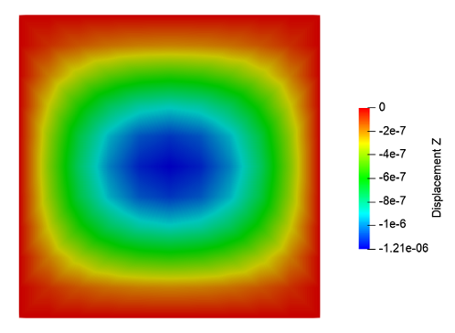
3. Check the numerical value of the maximum displacement.
Display maximum Component Z of the Displacement field. Select a point in the center of the square and display information about it.
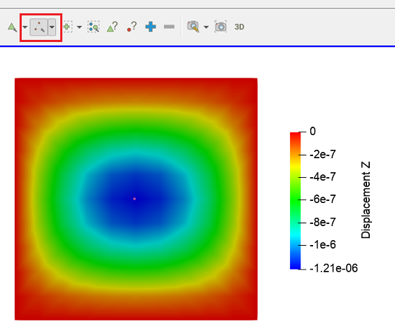
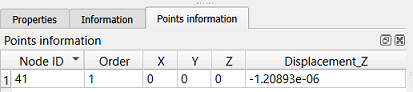
The difference between the resulting value 1.209e-6 and the required -1.19e-6 is 1.6%.
4. Check numeric values of moments in the center of the plate.
Display component XX of the MomentsShell field.
On the main FidesysViewer panel, select Filters – Alphabetical – Probe Location. In the Properties tab, specify the following values:
Center: (0,0,0);
Radius: 0;
Number Of Points: 1.
Click Apply.
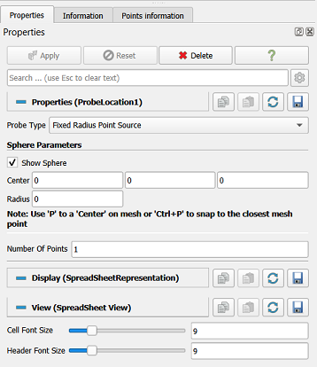
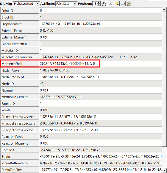
The difference between the resulting values (M x=260.347 and M y=344.745) and the required ( Mx=252 and M y=332) is 3.3% and 3.8%, relatively.
5. Open 3D-image of the shell.
 To display 3D-view of the beam cross section, set
the focus on the calculation title and click the button 3D-view in the
FidesysViewer standard line.
To display 3D-view of the beam cross section, set
the focus on the calculation title and click the button 3D-view in the
FidesysViewer standard line.
The system will open a new file *.pvd and you will be able to apply various filters to it and to view its deformed view.
Choose the new file example_3D.pvd in the Model Tree and display Filters - Alphabetical - Warp by Vector for it with the following fields values.

For this filter, on the Properties tab, set:
Vectors: Displacement;
Scale Factor: 2e5;
Click Apply.
The deformed view will be displayed, but the shell will be drawn with thickness.
In the top panel, select the calculation result data to display.

 To apply all of the filters changes automatically,
click Apply changes to parameters automatically on Command Panel.
To apply all of the filters changes automatically,
click Apply changes to parameters automatically on Command Panel.
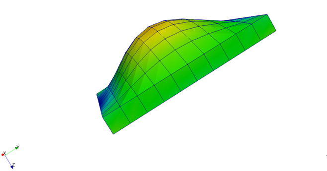
6. Download numerical data
Select File - Save Data in the Main Menu or click Ctrl+S. Enter the file name (*.csv format), leave it by default. Click OK. The saved file is an ordinary table of numerical data which can be opened in any text editor.
Geometry creating, meshing, setting boundary conditions and materials can be performed using the console interface. Below is a link to the program code that allows you to perform the steps described above manual, you only need to specify the full path and name.