Search the documentation
Enter at least 2 characters
Enter at least 2 characters
 |
CAE Fidesys 9.0 Documentation |
NAFEMS test “Thick Plate Pressure”, Test No LE10, Date/Issue 1990-06-15/2.
The problem of static load of a plate is being solved.
The pictures below represent a geometric model of the problem:
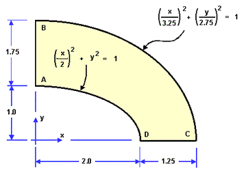
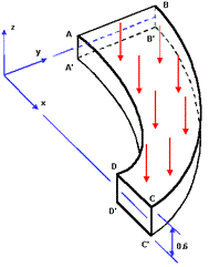
Displacements along the normal to the sides are constrained in the side slices of the plate. All of the points of the outer curvilinear surface are fixed in the XY plane. The outer curvilinear surface is fixed along the middle line of displacements along Z axis. The pressure to the upper side is 1 MPa. The material parameters are E = 210 hPa, n = 0.3.
Test pass criterion is the following: stress σyy at the point D is -5.38MPa to within 3%.
1. Create the first elliptic cylinder.
On the command bar, select the module for constructing volume geometry (Mode — Geometry, Entity — Volume, Action — Create).
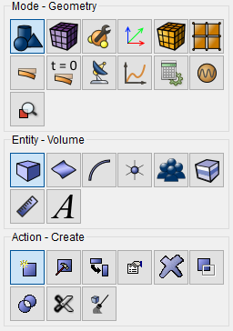
Select Cylinder in the list of geometric elements.
Specify the cylinder dimensions:
Height: 0.6;
Cross Section: Elliptical;
Major Radius: 2;
Minor Radius: 1.
Click Apply.
2. Create the second elliptic cylinder.
On the command bar, select the module for constructing volume geometry (Mode — Geometry, Entity — Volume, Action — Create). Select Cylinder in the list of geometric elements.
Specify the cylinder dimensions:
Height: 0.6;
Cross Section: Elliptical;
Major Radius: 3.25;
Minor Radius: 2.75.
Click Apply.
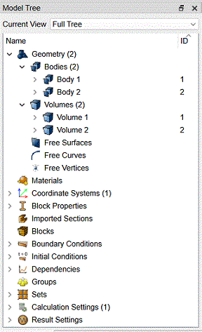
As a result, two generated entities are displayed in the Model Tree (Body 1 and Body 2):
3. Subtract the first cylinder from the second one.
On the command bar, select the module for constructing volume geometry (Mode — Geometry, Entity — Volume, Action — Boolean).
Select Subtract in the list of operations.
Set the following parameters:
A Volume ID(s): 2 (the volumes to be subtracted);
B Volume ID(s): 1 (volumes from which other volumes will be subtracted).0.60.
Click Apply.
As a result, only one volume is displayed in the Model Tree (Body 2).
4. Leave a quarter of a volume (symmetry of the problem).
On the command bar, select the module for constructing volume geometry (Mode — Geometry, Entity — Volume, Action — Webcut).
Select Coordinate Plane in the list of possible webcut types.
Set the following parameters:
Volume ID(s): 2 (the volume to be webcut);
Webcut with: YZ;
Offset Value: 0.
Click Apply.
Do the same for the ZX Plane:
Volume ID(s): 2 (the volume to be webcut);
Webcut with: ZX;
Offset Value: 0.
Click Apply.
As a result, the original volume in the Model Tree is split into three (Volume 2, Volume 3 and Volume 4).
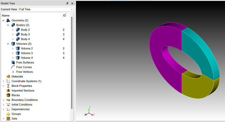
Delete the volumes 2 and 3. To do this, select these volumes in the Model Tree holding down Ctrl and click Delete in contextual menu. As a result, a quarter of the original volume is left (Volume 4).
5. Split the outer curvilinear surface into two (it is necessary for restraining this surface from displacements along the middle line).
On the command bar, select the module for constructing volume geometry (Mode — Geometry, Entity — Volume, Action — Webcut).
Select Coordinate Plane in the list of possible webcut types.
Set the following parameters:
Volume ID(s): 4 (volume to be cut);
Plane: XY;
Offset Value: 0;
Put a checkmark in the Merge box.
Click Apply.
The result will be two volumes 4 and 5 glued to each other along the
section plane: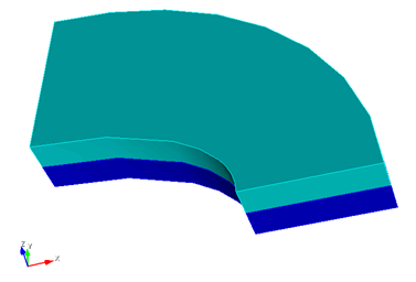
1. On the command bar, select the mesh module (Mode — Mesh, Entity — Curve, Action — Mesh).
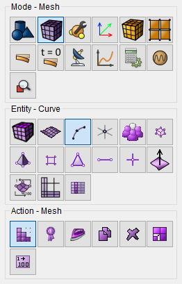
Specify the parameters of mesh refinement:
Select Curves: 43 44 45 46 (using space after each curve);
Select the way of meshing: Equal;
Select the checkbox Interval;
Specify the number of intervals: 12.
Click Apply Size.
Click Mesh.
2. On the command bar, select the mesh module (Mode — Mesh, Entity — Curve, Action — Mesh).
Specify the parameters of mesh refinement:
Select Curves: 12 14 39 41 (using space after each curve);
Select the way of meshing: Equal;
Select the checkbox Interval;
Specify the number of intervals: 8.
Click Apply Size.
Click Apply.
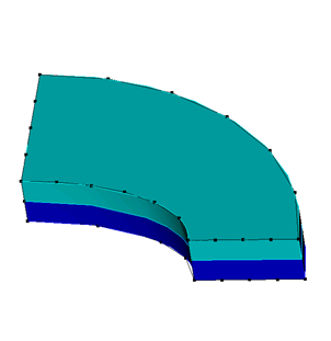
3. On the command bar, select the mesh module (Mode - Mesh, Entity - Curve, Action – Mesh).
Specify the parameters of mesh refinement:
Select Curves: 51 53 61 62 (through spaces);
Settings for Curve: Equal;
Select the checkbox Interval;
Specify the number of intervals: 2.
Click Apply Size.
Click Mesh.
4. On the command bar, select the volume mesh module (Mode — Mesh, Entity — Volume, Action — Mesh).
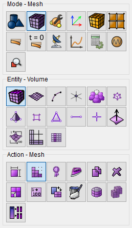
Specify the parameters of mesh refinement:
Select Meshing Scheme: Map;
Select Volumes: 4 5 (or by the command all).
Click Apply Scheme.
Click Mesh.
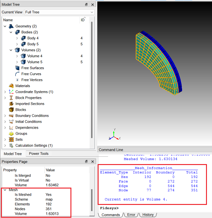
The resulting number of elements can be viewed in the Property Page by clicking on the inscription Volume 4 in the Model Tree on the left.
To view the mesh properties, you can follow these steps:
Select the entire model;
Right-click the model;
In the pop-up menu, select List Information – List Mesh Info;
Information on the mesh will be displayed in Command Line.
1. Fix one side (slice) along X axis.
On the command panel, select the boundary conditions module (Mode — Boundary Conditions, Entity — Displacement, Action — Create).
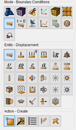
Set the following parameters:
Entity List: Surface;
Entity ID(s): 33 40;
Degrees of Freedom: X;
DOF Value: 0.
Click Apply.
2. Fix one side (slice) along Y axis.
On the command panel, select the boundary conditions module (Mode — Boundary Conditions, Entity — Displacement, Action — Create).
Set the following parameters:
Entity List: Surface;
Entity ID(s): 35 39;
Degrees of Freedom: Y.
Click Apply.
3. Fix the outer curvilinear surface along X and Y axes.
On the command panel, select the boundary conditions module (Mode — Boundary Conditions, Entity — Displacement, Action — Create).
Set the following parameters:
Entity List: Surface;
Entity ID(s): 36 38;
Degrees of Freedom: X and Y.
Click Apply.
4. Fix the middle line of the outer curvilinear side along Z axis.
On the command panel, select the boundary conditions module (Mode — Boundary Conditions, Entity — Displacement, Action — Create).
Set the following parameters:
Entity List: Curve;
Entity ID(s): 50;
Degrees of Freedom: Z.
Click Apply.
5. Apply pressure to the upper side.
On the command panel, select the boundary conditions module (Mode – Boundary Conditions, Entity – Pressure, Action – Create).
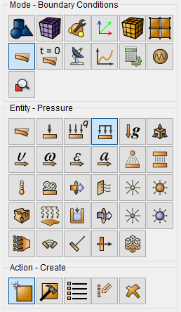
Set the following parameters:
Entity List: Surface;
Entity ID(s): 31;
Value: 1e6 (an exponential number format using the Latin letter“e” is supported).
Click Apply.
All applied boundary conditions must be displayed in the Model Tree on the left. In addition, the boundary conditions are available for editing from the Model Tree.
To view all the applied boundary conditions also click Show BC on the top panel.
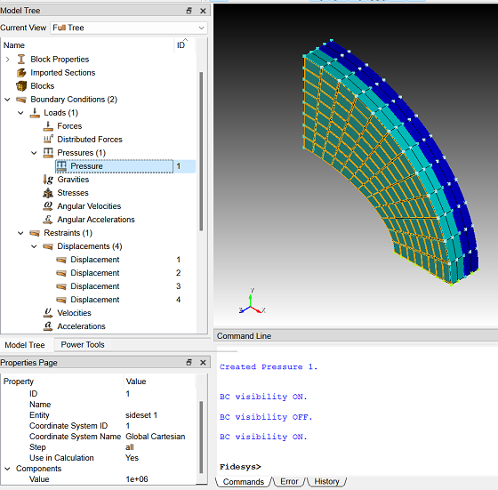
1. Create the material.
In the command bar, select the module for specifying material properties (Mode — Material, Entity — Materials Management).

In the Materials Management window that opens, in the second column, double-click on the caption. Enter the name of the material and write “Material 1”.
Click the ENTER key.
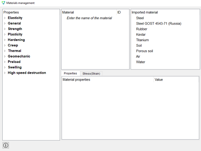
Next, using the “drag & drop” method, add the necessary characteristics from the left column to the Material Properties column.
In the left column, select Elasticity - Isotropic Material. Select with the mouse the characteristic Young's modulus. Hold down the left mouse button and drag the label to Material Properties. Double-click in the Value field opposite the Young's modulus and enter the number 2.1e+11.
Similarly, from the Isotropic Material section add the Poisson ratio 0.3.
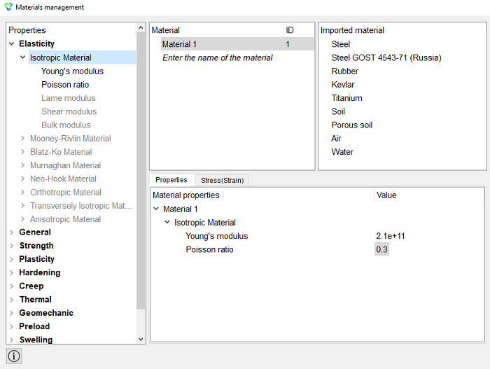
Click Apply.
Close the Materials management window.
2. Create a block of one type of the material.
On the command bar, select the block management module (Mode — Blocks, Entity — Block, Action — Add).

Set the following parameters:
Block ID: 1;
Entity List: Volume;
Entity ID(s): 4 5 (or by the command all).
Click Apply.
3. Set the block parameters.
On the command bar, select the block management module (Mode - Blocks, Entity - Block, Action - Block properties/parameters).

Set the following parameters:
Block ID(s): 1;
Category: Solid;
Material: Material 1;
Coordinate System: Global Cartesian;
Order: 2.
Click Apply.
1. Set the type of the problem to be solved.
On the command bar, select the calculation settings module (Mode — Calculation Settings, Calculation Settings — Static, Static — General).
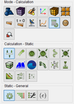
Select:
Dimension: 3D;
Model: Elasticity.
Click Apply.
2. Set the solver settings.
On the command bar, select the calculation settings module (Mode — Calculation Settings, Calculation Settings — Static, Static —Solver).
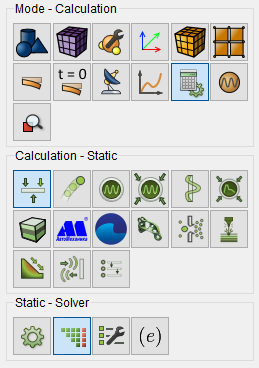
Select the solver method (direct or iterative) and set Convergence Parameters in case of choosing an iterative one. You can also leave all the settings by default.
Click Apply.
Click Start Calculation.
3. In a pop-up window select a folder to save the result and enter the file name.
4. In the case of a successful calculation, the console displays the message: Calculation finished successfully at "date" "time".
1. Open the file with the results. There are three ways to do that.
Click Ctrl+E.
From the main menu, select Calculation. Click Open Results.
Select Results on Command Panel (Mode - Results). Click Open results.

2. Display the component σyy of the stress field and the mesh on the model.
In FidesysViewer window set the following parameters on Toolbar:
Representation Field: Stress;
Representation Component: YY.
Surface With Edges.

3. Select a point where you need to view the stress.
Select a point on the model by using Select Points Through.

Select a point D on the upper side. From the main menu, select View – Selection Display Inspector.
In Selection Display Inspector, go to the tab Point Tag and select and click on the Stress line in the drop-down list.
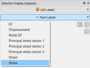
As a result, Stress components at the point D are displayed at the picture.
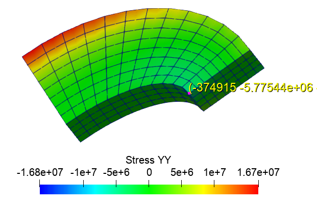
The difference between the obtained value -5.77577e+06 and the required one -5.380e+06 is 2%.
5. Download numerical data.
Select File → Save Data in the Main Menu or click Ctrl+S. Enter the file name (*.csv format), leave it by default. Click ОК. The saved file is an ordinary table of numerical data which can be opened in any text editor.
6. You can see the way the body is deformed under the applied pressure.
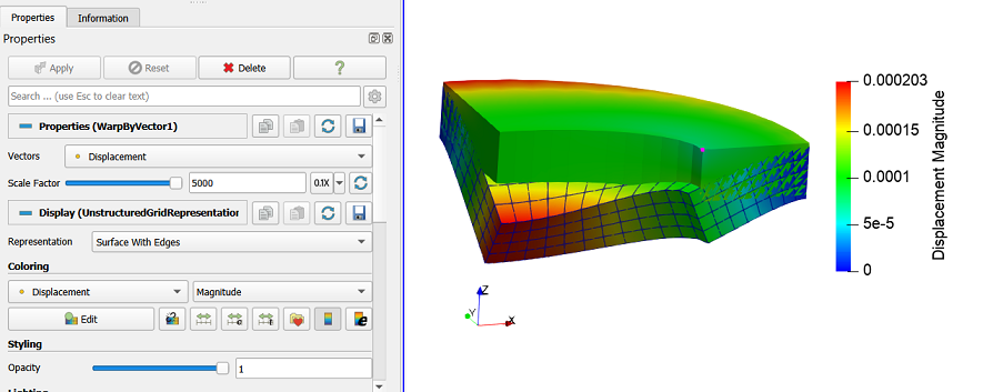
To do this select the filter Warp By Vector. Set the following parameters in the tab Properties: set the value to 5000 in the field Scale Factor.

As a result, the deformed body is displayed in the picture. To see the original model, click near it in the Model Tree. The picture below shows the deformed (solid grey filling) and the original model (with the field of displacements distribution along Y axis).
Geometry creating, meshing, setting boundary conditions and materials can be performed using the console interface. Below is a link to the program code that allows you to perform the steps described above manual, you only need to specify the full path and name.