Search the documentation
Enter at least 2 characters
Enter at least 2 characters
 |
CAE Fidesys 9.0 Documentation |
Definition (calculation) eigenfrequencies and eigenmodes (modal analysis) can be both an independent task of finite element analysis, and a necessary condition for performing dynamic time analysis using the decomposition of the desired solution by modes of natural oscillations, i.e. by the superposition method. Explanations of concepts natural frequency and the corresponding eigenmodes are given in the subsection Introduction based on the eigenvalues.
Calculation of eigenfrequencies and eigenmodes is started from the Command Panel (it is assumed that the user has already built a finite element the model of the analyzed object, including the set of boundary conditions).
Solver settings for static strength calculation are made from the Command Panel by selecting (Mode - Calculation Settings, Calculation Settings - Mode Frequency Analysis, ModeFrequency - General).
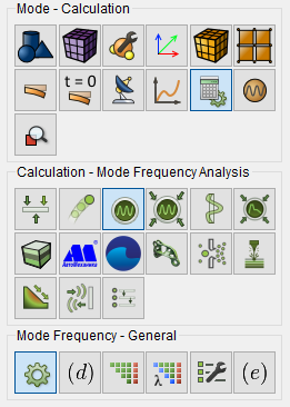
Fig. 1 - Command panel, general settings for mode frequency analysis
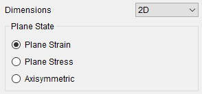
In the drop-down list Dimension select dimension the problem to be solved: 3D (three-dimensional; by default) or 2D (flat).
In the case of 2D in the radio button group Plane state select Plane strain or Plane stress:
In the Settings group, set the required to calculate the data: the number of determined eigenfrequencies and parameters their search (lowest values, target value, frequency range).
In the case of preloaded vibration analysis constructions check the box Preloaded model, and in the opened group Model specify the features such loading (plasticity, geometric nonlinearity, thermal conductivity).
Click Apply.
Solver settings for static strength calculation are made from the Command Panel by selecting (Mode - Calculation Settings, Calculation Settings - Mode Frequency Analysis, ModeFrequency - Output Fields) and perform the necessary solver settings.
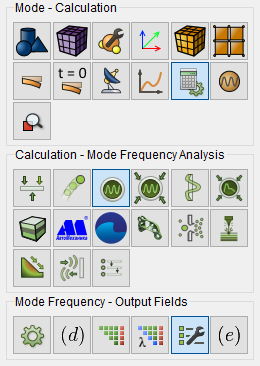
Fig. 2 - Command Panel, output field settings for modal analysis
The necessary information on this setting is given in the subsection Setting output fields of natural frequencies and forms.
Click Apply.
Click Start Calculation.
In a pop-up window select a folder to save the result and enter the file name.
In the case of a successful calculation, the console displays the message: Calculation finished successfully at "date" "time".
To display the calculation results, you can use icon  (Open the results of the last calculation). Clicking on this icon starts
the Fidesys postprocessor: Fidesys Viewer. A description of the operation
of this program is given in a separate manual.
(Open the results of the last calculation). Clicking on this icon starts
the Fidesys postprocessor: Fidesys Viewer. A description of the operation
of this program is given in a separate manual.
You can see examples of this calculation here: