Search the documentation
Enter at least 2 characters
Enter at least 2 characters
 |
CAE Fidesys 9.0 Documentation |
NAFEMS-Glasgow, BENCHMARK newsletter, Report No. E1261/R002, “Free Vibrations of a Simply-supported Thin Square Plate” , February 1989, p.21.
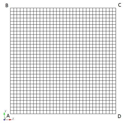
We solve the problem of modal analysis of a square plate.
The size of the plate is 10 m х 10 m, the thickness is 0.05 m. X- and Y-Translation and Z-Rotation are constrained for all nodes of the plate. All the edges are constrained in Z-direction. The X-rotation is constrained for edges AB and CD. The Y-rotation is constrained for edges BC and AD. The material parameters are E = 200 hPa, ν = 0.3, ρ = 8000 kg/m3.
We need to compare Eigenmodes from 1 to 8.
1. Create the plate.
On the command bar, select the module for constructing surface geometry (Mode — Geometry, Entity — Surface, Action — Create).
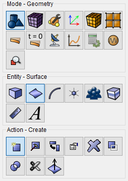
Select Rectangle in the list of geometric elements.
Set the brick dimensions:
Width: 10;
Location: ZPlane.
Click Apply.
A mesh of 32*32 linear quadrilateral elements is to be generated (as shown at the picture with the problem setting).
1. On the command bar, select the mesh module (Mode — Mesh, Entity — Curve, Action — Mesh).
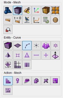
Specify the parameters of mesh refinement:
Select Curves: all;
Select the way of meshing: Equal;
Select splitting settings: Interval;
Interval: 32 (see the figure).
Click Apply Size.
Click Mesh.
2. On the command bar, select the surface mesh module (Mode — Mesh, Entity — Surface, Action — Mesh).
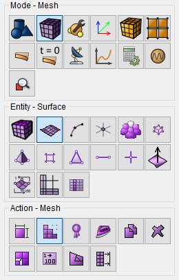
Select Meshing Scheme: Automatically Calculate;
Select Surfaces: 1 (or by the command all).
Click Apply Scheme.
Click Mesh.
1. Fix the plate: X- and Y-Translations and Z-Rotations.
On the command panel, select the boundary conditions module (Mode — Boundary Conditions, Entity — Displacement, Action — Create).
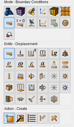
Set the following parameters:
Entity List: Node;
Entity ID(s): all;
Degrees of Freedom: X, Y and Z-Rotation.
Click Apply.
2. Fix all the edges at the Z-direction.
On the command panel, select the boundary conditions module (Mode — Boundary Conditions, Entity — Displacement, Action — Create).
Set the following parameters:
Entity List: Curve;
Entity ID(s): all;
Degrees of Freedom: Z.
Click Apply.
3. Fix the edges AB and CD on X-Rotation.
On the command panel, select the boundary conditions module (Mode — Boundary Conditions, Entity — Displacement, Action — Create).
Set the following parameters:
Entity List: Curve;
Entity ID(s): 2 4 (using space after each of them);
Degrees of Freedom: X-Rotation.
Click Apply.
4. Fix the edges BC and AD in Y-rotation.
On the command panel, select the boundary conditions module (Mode — Boundary Conditions, Entity — Displacement, Action — Create).
Set the following parameters:
Entity List: Curve;
Entity ID(s): 1 3 (using space after each of them);
Degrees of Freedom: Y-Rotation.
Click Apply.
1. Create the material.
In the command bar, select the module for specifying material properties (Mode — Material, Entity — Materials Management).

In the Materials Management window that opens, in the second column, click on the caption Enter the name of the material and write “Material1”.
Click the ENTER key.
In the left column, select Elasticity - Isotropic Material. Select with the mouse the characteristic Young's modulus. Hold down the left mouse button and drag the label to Material Properties. Double-click in the Value field next to Young’s modulus and enter the number 2e+11. Similarly from the Isotropic Material section add the Poisson ratio 0.3, Density: 8000.
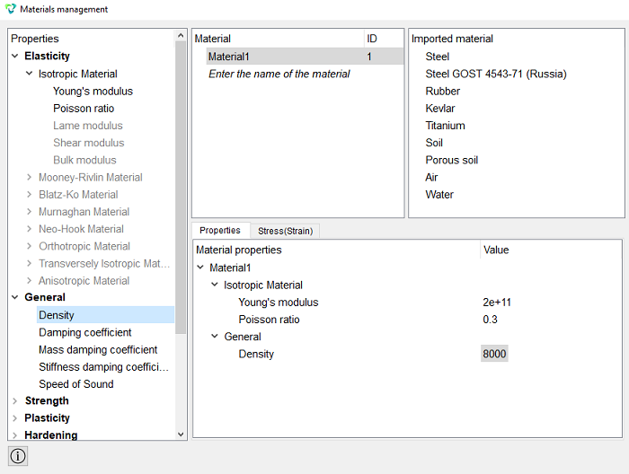
Click Apply.
Close the Materials management window.
2. Create the block of one type of the material
On the command bar, select the block management module (Mode — Blocks, Entity — Block, Action — Add).

Set the following parameters:
Block ID: 1;
Entity List: Surface;
Entity ID(s): 1 (or by the command all).
Click Apply.
3. Set the block parameters.
On the command bar, select the block management module (Mode - Blocks, Entity - Block, Action - Block properties/parameters).

Set the following parameters:
Block ID(s): 1;
Category: Shell;
Coordinate System: Global Cartesian;
Order: 1.
Set the shell properties by clicking the button  .
.
Set the following parameters:
Material: Material1;
Thickness: 0.05;
Eccentricity: 0.5.
Click Apply.
Close the window Set Shell Properties.
Click Apply.
1. Set the type of the problem to be solved.
On the command bar, select the calculation settings module (Mode — Calculation Settings, Calculation Settings — Mode Frequency Analysis, Mode Frequency — General).
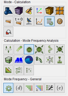
Leave all settings as default.
Set the default settings.
Click Apply.
Click Start Calculation.
2. In a pop-up window select a folder to save the result and enter the file name.
3. In the case of a successful calculation, the console displays the message: Calculation finished successfully at "date" "time", as well as the required eigenvalues and frequencies.
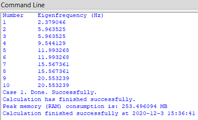
1. Compare the obtained results to those given in the picture.
Open the file with the results. There are three ways to do that.
Click Ctrl+E.
From the main menu, select Calculation. Click Open Results.
Select Results on Command Panel (Mode - Results). Click Open results.

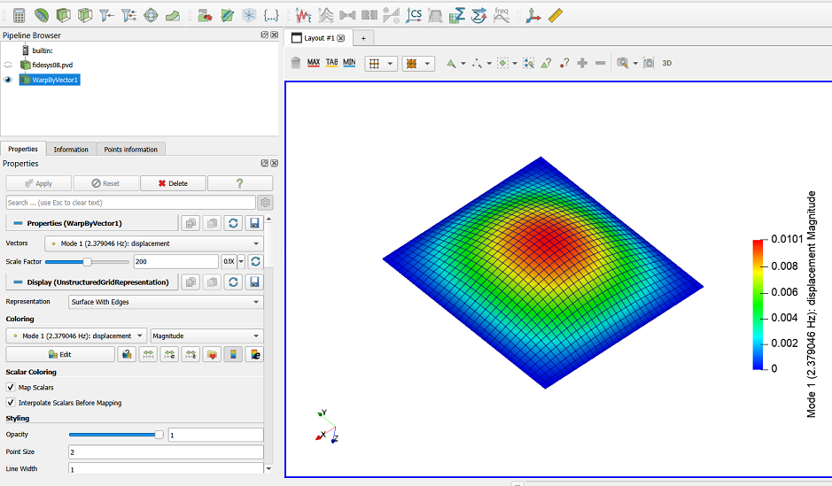
2. You can see the way the body is deformed under the applied pressure.
Select a filter Warp By Vector to do this.

Set the following parameters in the tab Properties:
Vectors: Moda 1 (2.379046 Hz): displacement;
Scale Factor: 200.
As a result, the deformed body is displayed at the picture. To see the original model, click near it in the Model Tree. The picture below shows the deformed model at different eigenvalues.

Geometry creating, meshing, setting boundary conditions and materials can be performed using the console interface. Below is a link to the program code that allows you to perform the steps described above manual, you only need to specify the full path and name.