Transient Analysis

Dynamic time analysis is the analysis of transients in mechanical systems that are excited by time-varying mechanical or thermal loads. Such an analysis can be carried out by direct solutions of the equations of dynamic equilibrium of the system in related coordinates or using the decomposition of the desired solution (in the case of mechanical loading - displacement) by the tones of natural vibrations, i.e. in normal (unrelated) coordinates. In both cases, integration is carried out solving equations in time using either explicit or implicit schemes.

For transient calculation, it is possible to save data in the format SEG-Y.

Transient analysis is started from the Command Panel (assumed, that the user has already built a finite element model of the analyzed object, set boundary conditions and loads):

The fields for displaying the results of dynamic time analysis are configured from the Command Panel by selecting (Mode - Calculation Settings, Calculation settings - Transient Analysis, Transient - General).

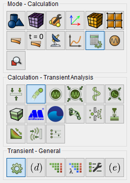
Fig. 1 - Command panel, general settings for transient analysis

In the drop-down list Dimension select dimension the problem to be solved: 3D (three-dimensional; by default) or 2D (flat).
In the case of 2D in the radio button group Type for a flat task select Plane stress or Plane strain:

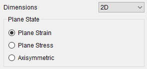
If necessary, you can use spectral element method; to do this, check the appropriate boxes.
In the drop-down list, select the method, depending on depending on the nature of the task, Full solution (direct solution in related coordinates; default) or Mode Superposition (solution in normal coordinates).

Further, in the form of steps 8 - 11, the actions when choosing a method are described Complete solution.

In the drop-down list Schema select Implicit (default) or Explicit.
For an implicit scheme, set the Settings in the group:
- the considered time interval of the transition process (in the input window Maximum time).
- the number of steps in time or the size of the step (using a suitable radio buttons).
In the group of flags Model check the box corresponding to features of the solution model used:
- Elasticity.
- Plasticity.
- Nonlinear geometry.
- Heat transfer.
- Pore Fluid Transfer.
In the case of a nonlinear problem (taking into account plasticity or geometric non-linearity) it is necessary to check the box To set the settings of the nonlinear solver. This will open the corresponding input windows:

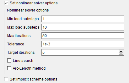
You can leave the default values in them, or specify required by the user.
Note: A system of nonlinear equations on each the time step is solved using Newton's iterative method, linear search or the method of bordering arcs (to select the last two, select the appropriate checkbox). When the specified accuracy of the solution or the maximum number of iterations is reached, the solution process is completed.

Regardless of the linear or nonlinear nature of the problem being solved, when using an implicit time integration scheme , it is necessary set its settings. To do this, select the checkbox to set implicit scheme settings and specify the attenuation of the Newmark algorithm in the corresponding input window:
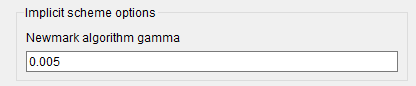
When selecting an explicit schema in the data group Settings you need to enter:
- maximum time;
- maximum number of steps in time.
Then, as for the implicit scheme, in the group Model you should specify the behavior model of the material or structural element (see above, step 9).

After that, select the checkbox to set the explicit scheme settings and specify the number of the Chime in the corresponding input window. or leave the default value:
Click Apply.

Settings for solving dynamic time problems by the superposition method.

If the superposition of the mod method was selected, then opens input window The number of mods in which you need to specify the corresponding value.
In the Settings group, set:
- maximum transition time;
- the number of steps in time or the step value.
In the case of vibration analysis of a preloaded structure, select the checkbox Preloaded model, and in the opened group Model specify the features of such loading (plasticity, geometric nonlinearity, thermal conductivity).
Note: When selecting the method Superposition The mod requires a preliminary determination of the eigenfrequencies and eigenmodes of the analyzed structure. If they were not previously determined, then the program recognizes the situation and launches the appropriate calculation is automatic.
Click Apply.

Further settings are made as follows:

On the Command Bar, among the time analysis settings, select icon (Transient analysis - Damping). This opens the input windows in which you need to set the appropriate values:
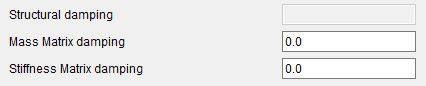
Click Apply.
On the Command Bar, among the time analysis settings, select icon (Transient Analysis - Solver) and perform the necessary solver settings.
Configure the output fields of the calculation results (Transient Analysis - Output Fields):

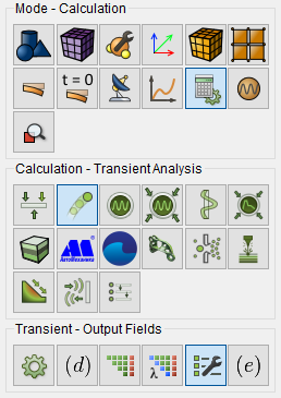
Fig. 2 - Command Panel, settings of output fields for temporary analysis

The necessary information on this setting is given in the subsection Configuring Output Fields in dynamic analysis.
Click Apply.
Click Start Calculation.

In a pop-up window select a folder to save the result and enter the file name.

In the case of a successful calculation, the console displays the message: Calculation finished successfully at "date" "time".

To display the calculation results, you can use the icon (Open the results of the last calculation). When you click the Fidesys postprocessor is launched on this icon: Fidesys Viewer. A description of the operation of this program is given in a separate manual.

You can see an example of this calculation here:

Dynamic loading.