Search the documentation
Enter at least 2 characters
Enter at least 2 characters
 |
CAE Fidesys 9.0 Documentation |
The 3D problem of 1D nonsteady heat transfer inside a beam is being solved.
The picture below represents a geometric model of the problem:
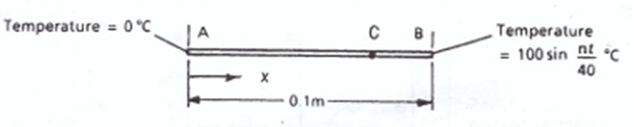
The beam length is 0.1 m, square cross section is 0.01x0.01 m. The temperature at the point A is TA = 0°C, the temperature at the point B varies harmonically: TB = 100 sin (πt/40)°C. The material parameters are isotropic, V = 35 W/(m·°C), C = 440.5 J/(kg·°C), ρ = 7200 kg/m3.
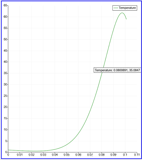
Test pass criterion is the following: temperature T at the point C (0.8;0;0) at time t = 32c is 36.60°C within 2%.
1. Create the sliver parallelepiped.
On the command bar, select the module for constructing volume geometry (Mode - Geometry, Entity - Volume, Action - Create).
Select Brick in the list of geometric elements.
Set the brick dimensions:
X (width): 0.1;
Y (height): 0.01;
Z (depth): 0.01.
Click Apply.
2. Combine left edge of the beam with the origin of coordinates.
On the command bar, select the module for constructing volume geometry (Mode - Geometry, Entity - Volume, Action - Transform).
Select Move in the list of possible types.
Set the following parameters:
Volume ID(s): 1;
Select Method: Distance;
X Distance: 0.05.
Click Apply.
1. Create the mesh of hexahedrons.
On the command bar, select the volume mesh module (Mode - Mesh, Entity - Volume, Action - Mesh).
The way of meshing: Polyhedron;
Select Volumes: 1 (or by the command all).
Click Apply Scheme.
2. Set the size of the elements.
On the command bar, select the volume mesh module (Mode - Mesh, Entity - Volume, Action - Intervals).
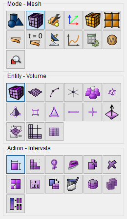
Specify the following parameters:
Select Approximate Size from the drop-down list;
Select Volumes: 1 (or with the all command);
Approximate Size: 0.001.
Click Apply Size.
Click Mesh.
1. Create the material
In the command bar, select the module for specifying material properties (Mode - Material, Entity - Materials Management).

In the Materials Management window that opens, in the second column, click on the caption Enter the name of the material and write “Material 1”. Click the ENTER key.
Set the following parameters:
Density: 7200;
Specific heat coefficient: 440.5;
Thermal conductivity coefficient: 35.
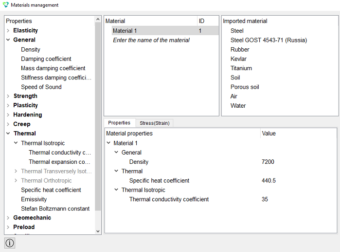
Click Apply.
Close the Materials management window.
2. Create a block of one type of the material.
On the command bar, select the block management module (Mode - Blocks, Entity - Block, Action - Add).

Set the following parameters:
Block ID: 1;
Entity List: Volume;
Entity ID(s): 1 (or by the command all).
Click Apply.
3. Set the block parameters.
On the command bar, select the block management module (Mode - Blocks, Entity - Block, Action - Block properties/parameters).

Set the following parameters:
Block ID(s): 1;
Category: Solid;
Material: Material 1;
Coordinate System: Global Cartesian;
Order: 1.
Click Apply.
1. Set the value of temperature applied to the left side of the beam.
On the command panel, select the boundary conditions module (Mode - Boundary Conditions, Entity - Temperature, Action - Create).
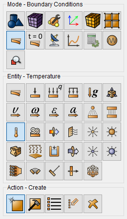
Set the following parameters:
Entity List: Surface;
Entity ID(s): 4;
Value: 0.
Click Apply.
2. Set the value of temperature applied to the right side of the beam.
On the command panel, select the boundary conditions module (Mode - Boundary Conditions, Entity - Temperature, Action - Create).
Set the following parameters:
Entity List: Surface;
Entity ID(s): 6;
Value: 1.
Click Apply.
1. Set time dependency of the temperature applied to the right edge of the beam.
Select (Mode - Boundary Conditions).
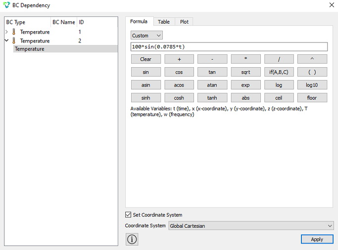
Click on the button Time dependency on Command Panel. The pop-up menu with the settings will be opened. On the left panel, select BC for which the time dependency will be set: Temperature 2.
Set the following parameters:
Time dependency type: Custom;
Enter formula: 100*sin(0.0785*t).
Click Apply.
1. Set the type of the problem to be solved.
On the command bar, select the calculation settings module (Mode — Calculation Settings, Calculation Settings — Transient analysis, Transient — General).
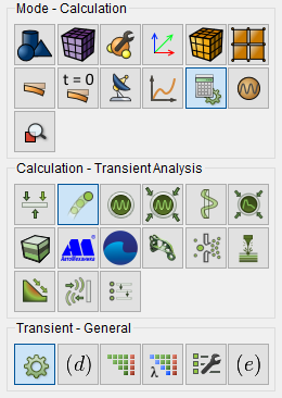
Set the following calculation parameters:
Dimension: 3D;
Method: Full Solution;
Scheme: Implicit;
Max Time: 32;
Steps Count: 100;
Elasticity: untick;
Heat Transfer: tick.
Click Apply.
Click Start Calculation.
2. In a pop-up window select a folder to save the result and enter the file name.
3. In the case of a successful calculation, the console displays the message: Calculation finished successfully at "date" "time".
1. Open the file with the results. There are three ways to do that.
Click Ctrl+E.
From the main menu, select Calculation. Click Open Results.
Select Results on Command Panel (Mode - Results). Click Open results.

You can see the calculation results in the pop-up FidesysViewer window.
2. There is a menu on Toolbar which allows viewing animation. It consists of a cycle of solutions calculated for every moment of time. Click Last Frame to see the model in time moment t = 32°C.

3. Display the component of the temperature.
In FidesysViewer window set the following parameters on Toolbar:
Representation Field: Temperature;
Representation Mode: Surface.

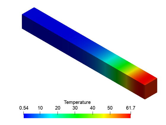
The model displays the mesh resulting from application of the spectral element method and the field of temperature distribution.
 To display the color legend scale, click the button
Toggle Color Legend Visibility on Command Panel.
To display the color legend scale, click the button
Toggle Color Legend Visibility on Command Panel.
4. To graph along one of the beam edges.
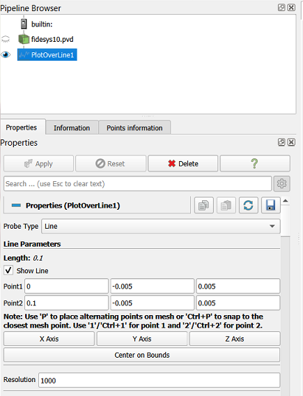
Select the filter Plot Over Line in the Main Menu. Set the coordinates of the points defining the line In the tab Properties:
Probe Type: Line;
Show Line;
Point 1 (coordinates): 0 -0.005 0.005;
Point 2 (coordinates): 0.1 -0.005 0.005;
Resolution: 100.
Click Apply.
 To apply all of the filters changes automatically,
click Apply changes to parameters automatically on Command Panel.
To apply all of the filters changes automatically,
click Apply changes to parameters automatically on Command Panel.
Click on the graph window appeared on the right side of the screen.
5. Display temperature change on the graph.
Click on the graph window, go to the tab "Display" in the filter control panel.
Set the Attribute Mode - Point Data
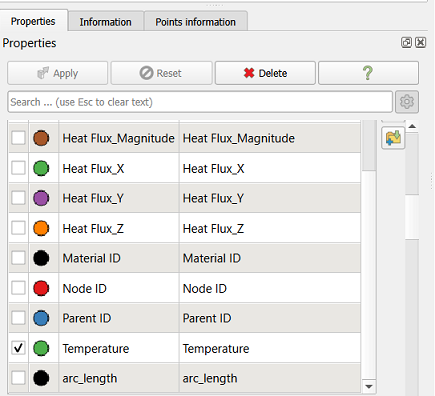
Next, in the field “Line Series”, set up labels against the parameters that you want to display on the graph.
Untick all the options except Temperature.
The temperature dependency at points belonging to the beam edge and the coordinates of these point coordinates are displayed on the graph.
6. Check the numerical temperature value T at the point (0.08;0;0).
Move the cursor to the required point on the graph. You can see a tool tip with the temperature value.
7. Download numerical data.
Select → File - Export in the Main Menu or click Ctrl+S. Enter the file name (*.csv format), leave it by default. Click OK. The saved file is an ordinary table of numerical data which can be opened in any text editor.
Geometry creating, meshing, setting boundary conditions and materials can be performed using the console interface. Below is a link to the program code that allows you to perform the steps described above manual, you only need to specify the full path and name.