Search the documentation
Enter at least 2 characters
Enter at least 2 characters
 |
CAE Fidesys 9.0 Documentation |
The angular velocity can be set for any type of geometric entity.
The creation or modification of such boundary conditions is carried out as follows:
On the Command Bar, select Mode - Boundary Conditions.
Select Entity - Angular Velocity.
Using graphical user interface elements specify the identifier (ID) or the name of the set of boundary conditions, specify entity that are subject to restrictions, determine the degrees freedoms and the magnitude of restrictions.
Click Apply.
The corresponding commands entered in the command prompt window, have the form:
[create] angular velocity [name <name>] [<id>] [{global|{add|on} {curve|node|nodeset|surface|vertex|volume} {[[id] {[<id>] [<id range start> to <id range finish>]}...] [all]}}]
modify angular velocity {[[id] {[<id>] [<id range start> to <id range finish>]}...] [<name>] [all]} [{global|{add|remove} {curve|node|nodeset|surface|vertex|volume} {[[id] {[<id>] [<id range start> to <id range finish>]}...] [all]}}]
[name <name>]
[dof <num> {value <value>|formula <formula id>|table <table id>|remove}] [cs {<ID>|<name>}]
[step {[[id] {[<id>] [<id range start> to <id range finish>]}...] [all]}]
The dof command determines the direction of the vector angular velocity. Values 1, 2 and 3 correspond to rotation around the axes X, Y and Z respectively.
This boundary condition is applied in statics and time analysis. Centripetal acceleration depends on the angular velocity according to:
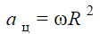
Thus, when using this GU, the final elements will be apply centripetal acceleration proportional to the square angular velocity.
The problem of rotation of a disk around its axis with a constant angular velocity is considered at a speed of 1 s(-1). The ring is fixed to the inner surface in the direction perpendicular to the plane (Z). Rotation angles are also prohibited relative to the axes lying in the plane of the ring (X,Y). The problem of time analysis is solved, the time interval is 5 s, the solution is in increments of 1 s.
Figure 2-3 shows the results - radial normal stresses and displacement (in cylindrical SC).
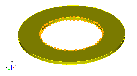
Figure 1 - Boundary conditions
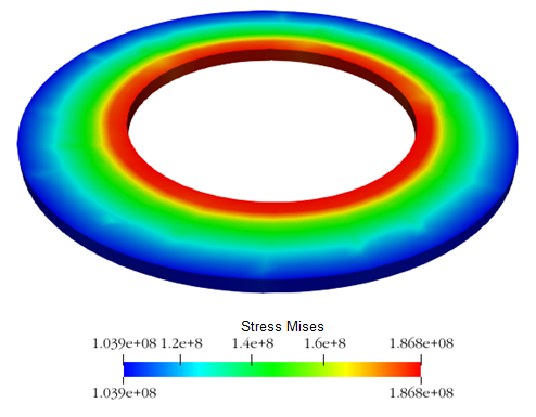
Figure 2 - Distribution of equivalent stresses, Pa
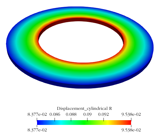
Figure 3 - Distribution of radial displacements, m