Search the documentation
Enter at least 2 characters
Enter at least 2 characters
 |
CAE Fidesys 9.0 Documentation |
To solve the problems of high-speed interaction of bodies (with speeds from 50 m/s to 20,000 m/s), taking into account the destruction and formation of fragments, a specialized computational core is used, which requires setting a certain minimum set of data to start the calculation. Such a minimum amount of data is the properties of materials for all bodies involved in the calculation according to the selected physical model described by one of the equations of state (URS), as well as the initial velocity of at least one of the bodies.
The computational core used supports finite element models with grids based only on triangular (for planar problems) and tetrahedral (for three-dimensional problems) finite elements of the 1st order.
The specifics of the computational core operation require setting the material constants in specific dimensions , shown in Tables 1-7. To match these dimensions , the geometric dimensions of the structure must be set in centimeters [cm], time in microseconds [mks], and speed in kilometers per second [km/s].
After applying the "High-speed destruction" analysis type with a check mark in the "Create configuration files before launch" field by clicking the "Apply" button, but before launching the calculation by clicking "Start calculation", in the "C:\Users\user_name\Documents\CAE-Fidesys-X.X " an hsdf folder is being created with preliminary versions of files for the calculation core - esmat.txt and data.txt , which contain the properties of materials and calculation settings that are available for additional editing before starting the calculation, which allows you to make edits to them and add additional directives to activate various calculation options. Additional directives can also be added via the corresponding "Additional Directives" field in the calculation settings. For a complete list of directives, see the section "Configuration File and directives" in the section "High-speed destruction".
When starting the calculation, the final versions of the files are generated in the directory specified for saving esmat.txt and data.txt , which contain the properties of materials and calculation settings that went into the calculation core.
In the case when the model contains bodies consisting of several blocks connected along the border, it is necessary to add the border_fusion directive to the calculation before starting, by activating the option "Merging the boundaries of different blocks".
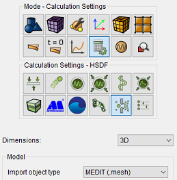
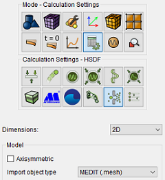
There is support for both two-dimensional (2D) plane and axisymmetric staging, as well as three-dimensional (3D).
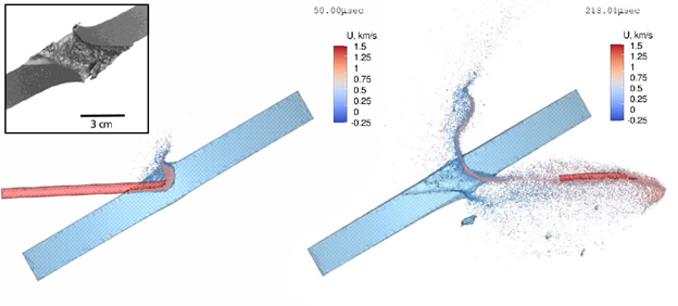
When applying any equation of state, first of all, it is necessary to specify the general physical and mechanical properties of the material, which include the parameters presented in Tables 1 and 2.
The variety of ways in which stresses and deformations can be changed, including different directions of force action, allows us to determine many types of elastic modulus. Table 2 shows three main modulus of elasticity, but since there are conversion formulas between them, it is enough to specify any 2 modulus of elasticity out of the 3 necessary ones.
| Обозначение в esmat.txt | Property | Dimension | Location |
| rho | Density | [g/cm3] | General – … |
| Y | Yield strength (tensile strength) | [GPa] | Plasticity – Mises Criterion – … |
| Designation in esmat.txt | Property | Dimension | Location |
| Ks | Adiabatic volume compression modulus (calculated automatically) | [GPa] | Elasticity – Isotropic Material – …
If not specified, it is calculated automatically using any two of the following values: Young's modulus (E), Poisson's ratio (nu), shear modulus (G) and the first parameter (modulus) Lame (λ) |
| G | Shear modulus | [GPa] | Elasticity – Isotropic Material – … |
| nu | Poisson ratio | - | Elasticity – Isotropic Material – … |
To solve the problem of high-speed interaction of bodies, it is necessary to use the equation of state of matter. The equation of state (URS) is a ratio reflecting, for a specific class of thermodynamic systems, the relationship between macroscopic physical quantities characterizing it, such as temperature, pressure, volume, chemical potential, entropy, internal energy, enthalpy, etc. URS is necessary to obtain specific results concerning the system under consideration using the mathematical apparatus of thermodynamics. These equations are not contained in the postulates of thermodynamics, so for each macroscopic object chosen for study, they are either determined empirically, or for the model of the system under study, they are found by methods of statistical physics. Within the framework of thermodynamics, the equations of state are considered to be set when defining a system.
Filling in the above structure describing the properties of materials begins with obtaining information from the reference literature on physical and mechanical properties, for example, [4]. The equation of state is calculated according to the method described above.
In the HSDF software module, it is possible to use several equations of state – simple and more complex, for example, a wide-range low-parameter equation of state. The software module determines which type of URS to use either automatically, using data on the number of specified constants, or explicitly specifying the type based on a specific set of material constants for the selected type.
In the software module, it is possible to explicitly specify several types of state equations, which are determined by a given set of constants – linear, feweos, poisson, lambda.
To use any URS, it is necessary to determine the physico-mechanical properties rho, Y, Ks, G, nu, defined in Tables 1 and 2:
– Type 1 (linear). Simplified, linear equation of state  . It is used, as a rule,
for new materials for which there is little data in the literature. To
use this URS, the properties rho, Y, Ks, G, nu from Tables 1 and
2 are sufficient. It is recommended to use it at interaction speeds of
no more than 1 km/s.
. It is used, as a rule,
for new materials for which there is little data in the literature. To
use this URS, the properties rho, Y, Ks, G, nu from Tables 1 and
2 are sufficient. It is recommended to use it at interaction speeds of
no more than 1 km/s.
– Type 2 (feweos). Thermodynamic low-parameter equation of state. This type of COURSE is recommended for use at high (cosmic) interaction speeds, operating in the temperature range up to 50,000 K and pressures up to 5,000,000 atmospheres. To use a low-parameter URS, it is necessary to specify in addition to the constants rho, Y, Ks, G, nu from Tables 1 and 2 the constants t, A, C, Eo, Cv, Ce, d2 from Table 3.
– Type 3 (poisson). A wide-range low-parameter equation of state with mechanical corrections. Similar to type 2, but takes into account changes in mechanical characteristics behind the shock wave front [3,4]. To use URS of this type, you must specify in addition to the constants rho, Y, Ks, G, nu, t, A, C, Eo, Cv, Ce, d2 from tables 1,2,3 add the constants nu_z, Pm from Table 4;
– Type 4 (lambda). The experimental equation of state, for calculation of the shock adiabatic through the Rankine–Hugonio ratio, taking into account the linear relationship of the shock wave velocity with the mass velocity:
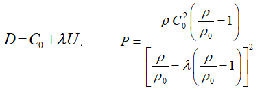
where D is the velocity of the shock wave, U is the mass velocity behind the shock wave front, p is the density, P is the pressure on the shock adiabate, C0 and λ are the parameters of the material. To use URS of this type, it is necessary to specify in addition to the constants rho, Y, Ks, G, nu from Table 1,2 – dependencies Co, lambda, d2 from Table 5. In general, it is recommended to use URS at interaction speeds of no more than 6 km/s.
| Designation in esmat.txt | Property | Dimension |
| Kt | Isothermal volume compression module (optional property, set optionally) | [GPa] |
| t | Type of quantum mechanical theory:
0 – for the Landau–Slater theory 1 – for the MacDonald–Douglas theory 2 – for the Zubarev–Vashchenko theory (the value is ignored and can be any) |
- |
| A | Constant A (calculation of cold pressure and energy for low-parameter URS) | - |
| С | The first, second and third constants of integration of cold pressure (and energy for low-parameter URS, three numbers are given) | - |
| Eo | Initial energy | [J/kg] |
| Cv | Heat capacity at constant volume | [J/kg K] |
| Ce | Electronic heat capacity | [J/kg K2] |
| Td | Debye temperature (optional property, set optionally) | [K] |
| Tm | Melting point(optional property, set optionally) | [K] |
| d2 | Compression ratio (at which “stitching” occurs with a linear equation of state (type 1) default value is 3) | - |
| Designation in esmat.txt | Property | Dimension |
| nu_z | The rate of change of the Poisson's ratio (from pressure, range (0,1]) | - |
| Pm | Melting pressure at the impact adiabate | [GPa] |
| Designation in esmat.txt | Property | Dimension |
| Co | The speed of sound, at P=0 | [km/s] |
| lambda | The experimental value of the tangent (the angle of inclination between the velocity of the shock wave and the mass velocity) | - |
| d2 | Compression ratio (at which “stitching” occurs with a linear equation of state (type 1) the default value is 3) | - |
To describe the destruction criteria, the constants from Table 6 are used. Also, to disable the destruction effect without removing the corresponding properties from the material, the nofracture directive is used, which is automatically added before the material properties in the file esmat.txt when activating the "Disable destructibility" option in the preprocessor before starting the calculation. A negative value for the destruction criteria means that there is no destruction according to this criterion.
All properties are located on the materials control panel in the branch "High–speed destruction - Destruction criteria – ..."
| Designation in esmat.txt | Property | Dimension |
| S1 | Ultimate strength(tensile strength) | [GPa] |
| S2 | Ultimate compressive strength (optional property, set optionally) | [GPa] |
| St | Ultimate shear strength (optional property, set optionally) | [GPa] |
| dS1 | Ultimate overstress (by default – 10%) | [%] |
| randS | Variance of ultimate strength (variance of deviation from the initial value of the maximum allowable tensile stress) | [%] |
| E1 | Ultimate strain (на растяжение) | [%] |
| E2 | Ultimate compressive strain | [%] |
| Et | Ultimate shear strain | [%] |
| dE | Ultimate overstrain (strain overvoltage, by default – 3%) | [%] |
| Wp | Plastic resilience (specific work on plastic deformations, optional property, set optionally) | [J/m3] |
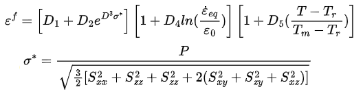
When using the Johnson-Cook model, you can also use the Johnson-Cook destruction limit parameter:
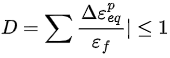
where ΔƐeqp - the increment of the intensity of plastic deformations in true coordinates, Ɛf is the plastic deformations of fracture.
If condition D>1 is met, we assume that the cell is destroyed.
| Designation in esmat.txt | Property | Dimension |
| Destruction from plastic deformations | ||
| jc_d1 | Initial destruction limit | - |
| jc_d2 | Coefficient of deformation failure | - |
| jc_d3 | The index of deformation failure | - |
| Destruction due to the rate of plastic deformation | ||
| jc_d4 | The coefficient of destruction depends on the rates of plastic deformation | - |
| jc_dе0 | The reference rate of deformation. (The default value is 1) | [1/]
|
| Destruction due to temperature influence | ||
| jc_d5 | The index of thermal destruction | - |
| To | Initial temperature | [K] |
| Tm | Melting temperature | [K] |
This parameter is only available for Johnson-Cook yield stress calculations.
The HSDF module implements the ability to select a simplified Johnson-Cook equation. To do this, the directives are grouped according to the multipliers included in the Johnson-Cook destruction equation. For example, if you set only directives from the group "Hardening from plastic deformations", then hardening from the rate of deformation and softening from temperature will not be taken into account. If all directives are selected, all multipliers of the equation will be taken into account.
The absence of a directive on the criterion of destruction means that there is no destruction according to this criterion.
To describe the hardening of a material, it is necessary to add the constants presented in Table 7 to the properties of the material. Using them, you can set a linear law of change in the yield strength from pressure for a single material, in accordance with the formula:
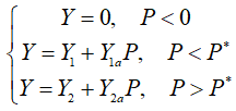
All properties except yield strength are located on the materials control panel in the branch "High–speed fracture Dynamic yield strength - ..."
| Designation in esmat.txt | Property | Dimension |
| Y | Yield strength (when stretched, under normal conditions) | [GPa] |
| Yap | First section tangent of angle(angle of inclination) | - |
| Y2P | Pressure changing the linear law (at which the linear law of change of the yield strength changes) | [GPa] |
| Y2ap | Second section tangent of angle (angle of inclination) | - |
| randY | Variance of yield strength (variance of deviation from the initial value of the yield strength) | [%] |
The CAE Fidesys HSDF software module implements the possibility of calculating the yield strength according to the Johnson-Cook model, taking into account dynamic hardening and softening. The Johnson-Cook Model:

where Yjc - he yield strength to be calculated from the model Johnson-Cook, Ɛeq - the equivalent true plastic deformation, έeq - is the rate of equivalent true plastic deformation, Т - he current temperature. The ability to choose a simplified one is also implemented. the Johnson-Cook equations. To do this, the directives are grouped in the table according to the multipliers included in the Johnson-Cook equation. For example, if you select only directives from the group "Hardening from plastic deformations", then hardening from the rate of deformation and softening from temperature will not be taken into account. If all directives are selected, all multipliers of the equation will be taken into account.
| Designation in esmat.txt | Property | Dimension |
| Hardening from plastic deformations | ||
| jc_A | Initial yield strength under static loading | [GPa]
|
| jc_B | Coefficient of deformation hardening | [GPa]
|
| jc_n | The index of deformation hardening | - |
| Hardening from the rate of plastic deformation | ||
| jc_C | A coefficient that takes into account the effect of the deformation rate | - |
| jc_dе0 | The reference rate of deformation. (The default value is 1) | [1/s]
|
| Softening due to temperature influence | ||
| jc_m | Thermal softening index | - |
| To | At what temperature the loading is set | [K] |
| Tm | Melting temperature | [K] |
The following properties are used to model the initial heterogeneity of material properties (in the state of supply) in terms of stress or yield strength:
randY – the property allows you to set Y (yield strength) in the volume of one body with a given variance from the initial value. To describe the yield strength deviation, it is necessary to use the andy property, the parameter can be specified in the form randY = n, where n is the specified deviation value, set within 0.01÷0.99, which means a deviation from the set value by 1% and 99%, respectively.
randS– the property allows you to set S1 (maximum allowable tensile stress) in the volume of one body with a given variance from the initial value. To describe the deviation of the permissible tensile stress, it is necessary to use the randS property, the parameter can be specified in the form randS = n, where n is the specified deviation value, set within 0.01÷0.99, which means a deviation from set values by 1% and 99%, respectively.
1. Kraus E.I., Shabalin I.I. A few-parameter equation of state of the condensed matter // J. Phys. Conf. Ser. 2016. Т. 774. С. 012009.
2. Kraus E.I. Low-parameter equation of state of a solid at high energy densities // Bulletin of NSU. 2007. Vol. 2, No. 2. P. 65–73.
3. Kraus E.I., Shabalin I.I. Calculation of elastic modules behind strong shock wave // J. Phys. Conf. Ser. 2015. Т. 653. С. 012085.
4. Kraus E.I., Shabalin I.I. A new model to determine the shear modulus and Poisson’s ratio of shock-compressed metals up to the melting point // High Press. Res. 2021. Т. 41, № 4. С. 353–365.
5. Tables of physical quantities. Handbook. / edited by Kikoin, Academician I.K. Moscow: Atomizdat, 1976. 1008 p.
6. Kraus E.I., Fomin V.M., Shabalin I.I. Model equations of thermodynamic functions of the state of substances. 2. Liquid and description of melting // Physical mesomechanics. 2004. Vol. 7. Pp. 289–292.
7. Fomin V.M., Kraus E.I., Shabalin I.I. A few-parameter equation of state of the condensed matter and its application to the impact problems // EPJ Web Conf. 2010. Т. 10. С. 00027.
8. Fomin V.M., Kraus E.I., Shabalin I.I. An equation of state for condensed matter behind intense shockwaves // Mater. Phys. Mech. 2004. Т. 7, № 1. С. 23–28.