Geometric Block

A geometric block of 2D geometry

This block defines geometric models of all the objects involved in the task. The geometry description block follows immediately after the initial data block., It starts with the start_geometry directive and ends with the end_geometry directive. Within these directives, the geometric configuration of all the bodies of the interaction object and its initial kinematic parameters are set. The configuration can be represented as simple geometric primitives: circle, polygon, ellipse, etc. and their combinations. It is necessary to take into account the fact that in the case of axial symmetry, only the upper half is given a geometric object. The order in which geometry is set inside a single body it matters because all operations are performed strictly sequentially. In general, directives for specifying geometric primitives have the following syntax:

the name of the directive (variable1, variable2, ...)

the number of variables and location in the directive must strictly match descriptions.

After the grid generation is completed, the results are recorded in the following for use in other tasks, thereby reducing generation time. grids in further calculations. The bodymesh.rbmf file is used to store the grid. which is located in the calculation's tmp directory (extension *.rbmf – this is the internal format of the grid storage package). Also in the same directory An element-by-element file of materials mat2mesh.rmmf is stored, linked to geometry. As a rule, this file is interesting to use in the future., for bodies consisting of heterogeneous materials. Thus, you can fix heterogeneity for all subsequent calculations of the same type and reduce time to generate heterogeneity. A materials file is used for storage. in the internal format *.rmmf. To reduce the amount of information stored , it is possible to use the storage directive.

body_speed is a directive that declares that a geometric The description of the body is finished. Despite the fact that the directive does not directly relate to the geometry of the calculated object, it is used as a placemark. the end of the body geometry construction. In addition, using this directive The kinematic initial data and the material are set. The directive uses the following variables:

body_speed (U,V,material)

U is the velocity of the body in the direction of the axis OX [km/s];

V is the velocity of the body in the direction of the axis of the motor control unit [km/s];

material – the number of the material from which the body is made (number you can find out the material by running the executable module with the option “--listmat”).

body_speedfile is a directive that declares that a geometric The description of the body is finished. The directive fully complies with the body_speed directive the only difference is that the material numbers are taken from the file. The Directive It is designed to specify the same heterogeneous materials when calculating the same type of tasks, but, for example, at different speeds. The directive uses the following variables:

body_speedfile (U,V,matfile)

U is the velocity of the body in the direction of the axis OX [km/s];

V is the velocity of the body in the direction of the axis of the motor control unit [km/s];

matfile is the path to the materials file with the extension *.rmmf.

body_mat is a directive that completely repeats the properties of the directive body_speed, with the only difference that the initial velocity is not set, but copied from the previous body. This directive is convenient to use for complex assemblies of bodies where the initial velocities are the same but different only materials. The directive uses the following variables:

body_mat (nmaterial)

nmaterial – the number of the material from which the body is made (number you can find out the material by running the executable module with the option “--listmat”).

body_matfile is a directive that declares that a geometric The description of the body is finished. The directive fully complies with the body_mat directive the only difference is that the material numbers are taken from the file. The Directive It is designed to specify the same heterogeneous materials when calculating the same type of tasks, but, for example, at different speeds. The directive uses the following variables:

body_mat (matfile)

matfile is the path to the materials file with the extension *.rmmf.

code is a directive that is designed to define the boundary of a body that has a common shared boundary with another body. This directive along with with a simpler interface for setting the boundary geometry, it automatically fills in an array of “neighboring borders". All bodies and their boundaries are numbered. Numbering tel – sequential through-line. Numbering of borders is sequential through within the body. The directive uses the following variables:

copygeom (nb,ng)

nb – body number;

ng is the border number of the copied body with the number nb.

If nb = -1, the number is calculated automatically and means “previous body".

If ng = -1, the number is calculated automatically and means “last border nb of the body”

Example:

To create a new border, you can use one of the following routines, described below, or if there is a common boundary between the bodies, simply copy the geometry data by calling the copygeom function. The Directive when copying, it reverses the border type and fills in the array. “contact boundaries", which reduces errors when setting a large the number of borders and facilitate the task of filling in the initial conditions of neighboring borders.

Calling copygeom(2,1) creates a new boundary and copies the data created by the routines krug, kvadrat, polygon, etc. from 1 boundary The 2nd body.

core is a directive that allows you to build a two–dimensional geometry the core of the projectile/impactor.

correct_step is a directive that is intended to be changed step through the space within the same body. In the initial block of the configuration file, the step is set (which is initially the same for all geometric primitives ). The use of a single step in the redistribution of the body is justified from the point of view of a single grid stiffness matrix, however, the use of the same The step value for all bodies of the calculated geometry is not justified from the point of view of estimated costs. The correct_step directive is used to set the multiplier to the base step, and this multiplier is valid within one body or until the next directive correct_step.

For example, the directive correct_step(2.0) increases the edge size triangular grid by a factor of 2, compared to the originally defined uniform step by step.

file is a directive that the software package uses to import the grid from the file. The HSDF module of the CAE Fidesys software package supports the following graphic formats *.rbmf, *.mesh, *.vtk, *.vol, *.ply, as well as CAD files*.step, *.igs, etc. Boolean operations on files they are not produced, so there is a limitation: one body – one file. The *.rbmf file is an internal grid format that is being created always in the process of completing a task, for each body and stored in tmp calculation directories. To reduce the amount of information stored , use the storage directive. The variables used are The following parameters:

file (geomfile, dx,dy,dz);

file (geomfile);

geomfile is the path to the file with the geometry and grid already calculated.

dx,dy,dz – after importing from the file, shift the coordinates of the geometry on (dx, dy, dz).

hardwall_coord(x,y,nx,ny) is a directive that defines the location of the “hard wall”. The directive uses the following variables:

x, y – installation coordinate;

nx, ny is the normal that determines the action of a rigid wall.

hardwall_glue_knots(nHW,type) is a directive that defines the method of movement of nodes located on a rigid wall. The directive uses the following variables:

nHW is the ordinal number of the rigid wall (-1 is the last wall);

type is the type of nodes that can be:

slide – slide knots along a rigid wall;

glue – glue the nodes to a rigid wall.

Attention!! To use the directive, you must first define the position of the rigid wall using the hardwall_coord directive.

Geometric block of 3D geometry

The principle of forming the configuration file remains the same, however it is necessary to disable all directives that do not apply to three-dimensional geometry. You can provide the program with ready-made three-dimensional calculations. models or generated computational grids based on ready-made three-dimensional models.

To switch to the three-dimensional geometry mode , specify the calc3d directive in the initial block of the configuration file. Also for The work must be specified in the system file or in the configuration file the geom3d directive, which explicitly tells the software package which 3D geometry builder to work with.

body_speed is a directive that declares that a geometric The description of the body is finished. Despite the fact that the directive does not directly relate to the geometry of the calculated object, it is used as a placemark. the end of the body geometry construction, i.e. it is this directive that defines, that ended the description of the body. This directive is used to set kinematic parameters. initial data. The directive uses the following variables:

body_speed (U, V, W, nmaterial)

U is the velocity of the body in the direction of the axis OX [km/s];

V is the velocity of the body in the direction of the axis of the motor control unit [km/s];

W is the velocity of the body in the direction of the OZ axis [km/s];

nmaterial – the number of the material from which the body is made (number you can find out the material by running the executable module with the “--listmat” option (see section 2).

body_speedfile (U,V,W,matfile)

U is the velocity of the body in the direction of the axis OX [km/s];

V is the velocity of the body in the direction of the axis of the motor control unit [km/s];

W is the velocity of the body in the direction of the OZ axis [km/s];

matfile is the path to the materials file with the *.rmmf extension.

body_mat – the directive is similar to the 2D case;

body_matfile – the directive is similar to the 2D case.

3.4.1 cadfile is a directive that allows you to import three–dimensional models built in CAD editors. The variables used are The following parameters:

cadfile(geomfile);

cadfile(geomfile, i_clock);

cadfile(vertex(dx, dy, dz), geomfile,);

cadfile(vertex(dx, dy, dz), geomfile, i_clock);

cadfile(vertex(dx, dy, dz), vector(x, y, z), α, geomfile);

cadfile(vertex(dx, dy, dz), vector(x, y, z), α, geomfile, i_clock).

geomfile is the path to the geometry file.

vertex(dx, dy, dz) is the reference point of the local coordinate system (if the local coordinate system is not specified, then the local coordinate system is coincides with the global Cartesian coordinate system (0,0,0));

vector(x, y, z) is the vector relative to which the rotation takes place (if the vector is not specified, the value (1,0,0) is used);

α is the angle of rotation.

i_block – border type ([1]- external| [-1] -internal) (if if the border type is not specified, then the value – external border is used).

In cases where geometry cannot be described by built-in geometric primitives or combinations thereof, you can use any other a program designed to build three-dimensional models of more complex designs and import them in the format “.igs” or “.step” for further calculation, as shown in Figure 1. The software package CAE Fidesys with HSDF module supports graphic formats CAD files *.step, *.igs, etc.

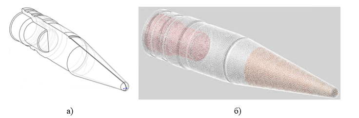
Figure 1 is the result of the geometry imported from SolidWorks

hardwall_coord(x,y,z,nx,ny,nz) is a directive that defines coordinates of the installation of the rigid wall. The directive uses the following variables:

x,y,z – installation coordinate;

nx, ny, nz is the normal that determines the action of a rigid wall.

hardwall_glue_knots(nHW,type) is a directive that defines the method of movement of nodes located on a rigid wall. The directive uses the following variables:

nHW is the ordinal number of the rigid wall (-1 is the last wall);

type is the type of nodes that can be:

slide – slide knots along a rigid wall;

glue – glue the nodes to a rigid wall.

Attention!! To use the directive, you must first define the position of the rigid wall using the hardwall_coord directive.

Literature

1. Sutherland I.E., Hodgman G.W. Reentrant polygon clipping // Commun. ACM. 1974. Vol. 17, № 1. P. 32–42.

2. Kraus E.I., Shabalin I.I., Shabalin T.I. Automatic tetrahedral mesh generation for impact computations // AIP Conference Proceedings. 2017. Vol. 1893. P. 030129.

3. Andreev A.N., Kraus E.I., Shabalin I.I. etc. Mechanics - from discrete to the continuous one. -Novosibirsk: Publishing house of the SB RAS, 2008. -344 p. Novosibirsk: Publishing house SB RAS, 2008. 344 p.

4. Kraus E.I., Fomin V.M., Shabalin I.I. Simulation of the collision process complex two-dimensional bodies against a deformable obstacle // Computational technologies. 2006. Vol. 11. P. 104–107.

5. Kraus E.I., Kraus A.E., Shabalin I.I. The Influence of the Contact Boundary in a Metal Matrix Composite on Dynamic Loading // Springer Proceedings in Physics. 2024. Vol. 1067 SPPHY, № November. P. 134–142.

6. Kraus E.I., Fomin V.M., Shabalin I.I. Dynamic construction method triangular meshes in multiply connected areas // Computational technologies. 2009. Vol. 14, No. 5. P. 40–48.

7. Shimada K., Gossard D.C. Bubble mesh // Proceedings of the third ACM symposium on Solid modeling and applications - SMA ’95. New York, USA: ACM Press, 1995. P. 409–419.

8. Conway J.H., Torquato S. Packing, tiling, and covering with tetrahedra // Proc. Natl. Acad. Sci. 2006. Vol. 103, № 28. P. 10612–10617.

9. Joe B. Geompack — a software package for the generation of meshes using geometric algorithms // Adv. Eng. Softw. Work. Elsevier, 1991. Vol. 13, № 5–6. P. 325–331.

10. Barber C.B., Dobkin D.P., Huhdanpaa H. The quickhull algorithm for convex hulls // ACM Trans. Math. Softw. 1996. Vol. 22, № 4. P. 469–483.

11. Si H. TetGen, a Delaunay-Based Quality Tetrahedral Mesh Generator // ACM Trans. Math. Softw. 2015. Vol. 41, № 2. P. 1–36.

12. Shewchuk J.R. Triangle: Engineering a 2D quality mesh generator and Delaunay triangulator. 1996. P. 203–222.

13. Johnson G.R., Beissel S.R., Gerlach C.A. A 3D combined particle-element method for intense impulsive loading computations involving severe distortions // Int. J. Impact Eng. Pergamon, 2015. Vol. 84. P. 171–180.

14. Kraus E.I., Shabalin I.I. Reactor2D: A tool for simulation of shock deformation // AIP Conf. Proc. 2016. Vol. 1770. P. 030092.

15. Petrov I.B. et al. About the combined method for numerical solution dynamic spatial elastoplastic problems // Academy Reports Sci. 2015. Vol. 460, No. 4. P. 389–391.

16. Wilkins M.L. Calculation of elastoplastic flows // Computational methods in hydrodynamics / ed. Older B., Fernbach S., Rotenberg M. Moscow: World, 1967. P. 212–263.

17. Official website of the bzip2 library.

18. Kraus A. et al. Numerical Modelling of High-Speed Loading of Periodic Interpenetrating Heterogeneous Media with Adapted Mesostructure // Appl. Sci. 2023. Vol. 13, № 12. P. 7187.

19. Tables of physical quantities. Directory. /ed. Kikoina acad. I.K. Moscow: Atomizdat, 1976. 1008 p.

20. Kraus E.I., Fomin V.M., Shabalin I.I. Model thermodynamic equations functions of the state of substances. 2. Liquid and description of melting // Physical mesomechanics. 2004. Vol. 7. P. 289–292.

21. Fomin V.M., Kraus E.I., Shabalin I.I. A few-parameter equation of state of the condensed matter and its application to the impact problems // EPJ Web Conf. 2010. Vol. 10. P. 00027.

22. Fomin V.M., Kraus E.I., Shabalin I.I. An equation of state for condensed matter behind intense shockwaves // Mater. Phys. Mech. 2004. Vol. 7, № 1. P. 23–28.

23. Kraus E.I. Few-parameter equation of state of a solid at high energy densities // Bulletin of NSU. 2007. Vol. 2, No. 2. P. 65–73.

24. Kraus E.I., Shabalin I.I. A few-parameter equation of state of the condensed matter // J. Phys. Conf. Ser. 2016. Vol. 774. P. 012009.

25. Kraus E.I., Shabalin I.I. Calculation of elastic modules behind strong shock wave // J. Phys. Conf. Ser. 2015. Vol. 653. P. 012085.

26. Kraus E.I., Shabalin I.I. A new model to determine the shear modulus and Poisson’s ratio of shock-compressed metals up to the melting point // High Press. Res. 2021. Vol. 41, № 4. P. 353–365.

27. Marsh S.P. LASL Shock Hugoniot Data // Los Alamos Series on Dynamic Material Properties. Univ of California Press, 1980. 150 p.

28. Trunin R.F. et al. Experimental data on shock wave compression and adiabatic expansion of condensed matter / ed. Trunina R.F. Sarov: RFNC-VNIIEF, 2006. 531 p.

29. Kinslow R., ed. High-velocity impact phenomena / ed. Nikolaevsky V.N. Moscow: Mir, 1973. 533 p.

30. Kraus E.I., Fomin V.M., Shabalin I.I. Accounting for electronic components in the equation of state when calculating shock waves in a mixture of metals // Vestnik Perm National Research Polytechnic University. Mechanics. 2001. No. 9. P. 78–84.

31. Kraus E.I., Shabalin I.I., Shabalin T.I. Numerical analysis of wave propagation in a cermet composite // AIP Conference Proceedings. 2017. Vol. 1893. P. 030130.

32. Fomin V.M. et al. Accounting for Functions of Distribution of Mechanical Properties of Metals in Dynamic Processes of Deformation and Destruction of Barriers // J. Eng. Phys. Thermophys. Springer, 2022. Vol. 95, № 7. P. 1–9.