CAE Fidesys 9.0 Documentation

Initial Data Block

In the initial block, the sequence of directives does not matter, and may The following directives are used:

add_time - directive that sets an additional period output for printing, is set together with the time directive. Used to change the established uniform printing step, in a given range.

add_time(t1, t2, dt)

t1 - initial time [μs];

t2 - final time [μs];

dt - period of printing [μs].

Example: add_time(12,19,0.01) means that at the moment time from 12 μs to 19 μs, step of printing results calculation is equal to 0.01 μs.

auto_step(ibody) - setting the grid step size according to acoustic impedance, ibody - body number, the grid size relative to which the mesh size will be calculated for other geometric bodies if ibody=0, then the body (material) is automatically searched with a minimum impedance and relative to it is calculated for other bodies. To build bodies taking into account impedance, you need to put correct_step in front of the body (negative number). This option is intended for developers, not recommended for use.

boolean = (delaunay|libgpc|gpc) – directive, using which defines the way boundaries are joined in 2D geometry (polygons). Boolean operations on polygons are a set of Boolean operations (AND, OR, NOT, XOR, ...) with one or more sets of polygons in computer graphics.These sets of operations are used in the software package to define geometry from primitives. In the software module of the computing geometry, the main objects are described using flat polygons. Operations of constructing a union, intersection or difference of polygons, despite Despite their apparent simplicity of formulation, they are very difficult to implement. Many existing implementation algorithms have significant drawbacks for practical use. The main problem is related to the loss of computing power accuracy when calculating the intersections of figures, which leads to incorrect the work of algorithms. In many algorithms, eliminating this kind of problem with accuracy leads to a significant complication of the algorithm implementation. Because today there is not a single algorithm that provides 100% correct execution, then several algorithms are implemented in the software module simultaneously. The directive can take one of three values:

delaunay – implements the Sutherland-Hodgman algorithm. This one of the very first and simplest polygon cutting algorithms [1]. This algorithm cuts the original general polygon with any convex polygon. A clipping polygon is usually called a clipping window . The essence of the algorithm is that the clipped polygon is sequentially clipped each edge of the cut-off window. The algorithm processes the intersection of each edges of the original polygon with each edge of the cutter, preserving the vertices, ribs located inside, and the points of intersection of the ribs. Then the algorithm is repeated, the temporary polygon obtained at the previous step is fed to the input and another edge of the cutter;

gpc – uses the gpc software module that implements Boolean operations using Vatti's algorithm. To use this command on your equipment must have the appropriate program preinstalled (project page http://www.cs.man.ac.uk/~toby/alan/software/). Mandatory the requirement is to set the path to the executable program module in configuration file;

libgpc – uses a built-in library based on gpc (http://www.cs.man.ac.uk/~toby/alan/software/), which implements Boolean operations through the Vatti algorithm (used by default).

bubble_mesh = (clists|verlet|delaunay|openmp|gpu|auto) – a directive that specifies the algorithm for implementing dynamic construction triangular mesh. The operating algorithm is described in [2,3]. The Directive may take one of the existing values:

clists – algorithm for constructing a mesh with repulsive-attractive potentially using a linked list of cells to speed up calculations (https://en.wikipedia.org/wiki/Cell_lists) and OpenMP parallel technologies;

verlet – algorithm for constructing a mesh with repulsive-attractive potentially using the Verley neighbor list to speed up calculations (https://en.wikipedia.org/wiki/Verlet_list) and parallel technologies OpenMP;

delaunay – algorithm for constructing a mesh with repulsive-attractive potential, with the determination of forces along the edges of the Delaunay triangulation. Method providing the highest possible mesh quality, but extremely slow due to the impossibility application of parallel technologies;

openmp – algorithm for constructing a mesh with repulsive potential using OpenMP parallel technologies for acceleration;

gpu – algorithm for constructing a mesh with repulsive potential using CUDA parallel technologies for acceleration;

auto – алгоритм определяется внутри программы исходя из начальных данных и заданной геометрии.

Default – auto.

Algorithms for dynamic meshing are described in more detail in [3,4].

bm_opt – directive that allows you to change default values for the methods for constructing a triangular and/or tetrahedral mesh described in 1.2.4. This directive is intended more for program developers, since setting variables is not trivial. The Directive uses the following variables:

bm_opt(bm_radius);

bm_opt(bm_radius,bm_stop);

bm_opt(bm_radius,bm_stop,bm_u_init);

bm_opt(bm_radius,bm_stop,bm_u_init,bm_cellrat);

bm_radius – sets the radius of the potential (radius cutoff), see Figure 1. It can take a value in the range from (1-1.5]. At a small value, only a repulsive potential is obtained. Default value -1.2;

bm_stop – value of the criterion for stopping the execution of the bubble_mesh algorithm (part of a step, maximum distance/step). The criterion indirectly determines number of integration steps in the equation of motion of grid nodes. Meaning default is 0.01(i.e. the maximum movement of any grid node, per one time step, cannot exceed one hundredth of a step);

bm_u_init – determines whether an initial random should be applied distribution of the speed value in mesh nodes. Can apply value– 0 (no) or 1 (yes). The default value is 0 (i.e. the initial the speed at grid nodes has a zero value);

bm_cellrat - determines the window size in the “cell lists” algorithm. The value is specified as a multiplier to the cutoff radius in the potential and can take a value in the range (1-50]. The parameter affects only the speed execution of parallel code in OpenMP and does not affect the quality in any way the resulting mesh. The default value is 1.6;

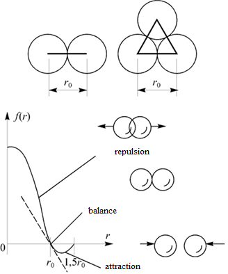
Figure 1 Type of particle interaction force

border_fusion – a directive that declares the need glue the boundaries of bodies that are in contact at the geometry stage, schematically this is shown in Figure 2. This directive sets the condition for ideal contact between two adjacent bodies. “Gluing” the contact boundary occurs when the following conditions are met:

• contact boundaries coincide “knot to knot”;

• the velocities of the nodes on the contact boundary coincide.  

The directive is usually used to specify heterogeneous environments, with a smooth contact boundary, an example of use is presented in [5].

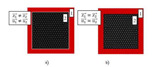
Figure 2 – Boundary conditions with sliding node(a);

Boundary conditions specified by the directive border_fusion (b)

You need to be aware that the directive does not work correctly in 3D tasks since condition 1 may not be met when constructing individual figures.

Default – “noborder_fusion”.

calc_file – directive that specifies the file name to write to calculation results, in which, in the format necessary for post-processing software, the result of the calculation at the last point in time will be presented.

All intermediate calculation results will be written to files with the modified name, including the print output number. All these files are recorded to the working directory work_dir.

condition_dump – directive that defines conditions when executing which the file dump_file is created. The Directive uses the following variables:

condition_dump(time, system, step, fracture)

time – calculation time in the running task [μs];

system – time spent by the processor on task calculations [min];

step – number of time steps [pcs];

fracture – percentage of destroyed cells [%] (1-100).

The dump_file file is created when one of the 4 conditions stated above. The fulfillment of conditions is counted from the beginning task start or the last time the dump_file was saved. All intermediate dump results will be written to files with a changed name, including the dump serial number (for example, dump.0001, dump.0002 etc.). At the end of the calculation, the file dump_file is always created, regardless of the established conditions.

The directive may not be specified - the default is “200,90,200000,1”, those. the file is created provided that the calculation of the 200 μs task has been carried out, or 1.5 hours of real time have passed, or the task has counted 200 thousand steps by time, or 1% destruction of bodies occurred. Current values ​​can be see in the command line, similar toFigure 2.

contact_algorithm = i – this directive defines the calculation method forces at the contact boundary. You can use one of the ones below values:

0 – slow contact symmetric algorithm;

1 – fast, pre-sorted, symmetric algorithm calculation of contact boundaries (used by default);

2 – fast calculation, symmetric algorithm with Gordon extension To Johnson;

3 – fast calculation, non-symmetric algorithm with software extension To Gordon Johnson;

6 – an algorithm with a preliminary calculation of forces, complete conservation pulse (unstable, may lead to local explosions in the calculation);

By default – contact_algorithm = 1.

contact_iteration = i is a directive that sets the number of iterations when calculating forces at the contact boundary, where i - the number of iterations. Missing since version 0.24.

By default – contact_iteration = 1.

crystal = (bcc|fcc|hcp|tet) is a directive that defines the method of creating a majority volume and filling it with initially placed mesh nodes in 3D geometry.

The choice of the majority volume and its filling with the initially placed mesh nodes in the spatial case is similar to the planar problem.

A complex technical object created using geometric primitives it sinks into the majority volume. This task is performed by the creation of a rectangular area with a high-quality homogeneous mesh. The lengths of the sides of a rectangular area, which are determined by the maximum dimensions of the technical object under study. Created using geometric primitives. The object sinks into the majoring volume. As in the flat case, the initial arrangement of nodes for a dynamic method of creating tetrahedral meshs determines the final quality and speed of the mesh construction [6,7]. As a basis The initial arrangement of nodes in three-dimensional space involves different types of crystal lattice in a solid, since it is impossible to fill an arbitrary body with ideal tetrahedra.

The majority rectangular area is filled with one of the types of crystal lattice, namely, face-centered (Figure 3a), volume-centered (Figure 3b), hexagonal (Figure 3b) and mixed tetra (Figure 3g) structures. The latter type creates a more perfect a tetrastructure that provides high-quality mesh. Algorithm details It was considered in [8], and an example is shown in Figure 3g, nodes 2 and 3 are replaced. nodes 4, which are located in the middle of short line segments connecting nodes 2 and 3.

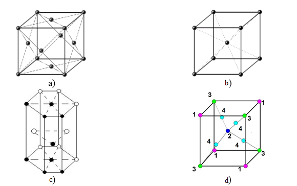
Figure 3 – Filling the majority area with the originally placed mesh nodes:

a) face-centered; b) volume-centered;

c) hexagonal; d) enhanced tetrastructure

Filling of the majority area is carried out by one of the existing directives:

bcc is the volume–centered structure of the crystal lattice;

fcc is the face–centric structure of the crystal lattice;

hcp is the hexagonal structure of the crystal lattice;

tet is a mixed tetra structure (default value).

debris is a directive that requires the calculation of fragmentation fields. Quite often, it is required to perform calculations in the process of solving problems. and the construction of a histogram of the distribution of fragments by velocity, mass, To control the parameters of fragment counting , algorithms have been developed for the differentiated output of information related to the visualization of the sizes and velocities of the fragmentation field. Additional directives are described below with a wide range of options.

The default is nodebris, a directive that specifies not to count shards.

debris_body(body1,body2,... bodyn) is a directive that defines the body numbers for which the fragments need to be counted body1, body2, ... bodyn. The numbering of bodies is continuous, as the geometry is specified in the configuration file.

To count fragments in all bodies, you must specify debris_body(0). The default value.

debris_box_auto(nbox) is a directive that determines that when when constructing the distribution of fragments, use uniform “boxes” over the entire range of fragment sizes, with a given number of "boxes". The size of the “box” (the size of the fragment) is automatically formed from zero size, up to the maximum size of the fragment. The directive uses variables:

nbox – the number of “boxes".

debris_box_manual(box1,box2,box3....boxn) is a directive that determines that when building a shard allocation, you must use arbitrary “boxes" of the specified size. The directive uses variables:

box1 – the minimum, first limiting size of the fragment;

box2 is the second limiting size of the shard, box2> box1;

….

boxn is the maximum, last limiting size of the shard.

debris_box_range(min_size,max_size,nbox) is a directive that determines that when building a shard allocation, you must use uniform “boxes" for fragments (with a selected range of fragment sizes). For visualization, only those fragments that fall will be shown. in the size range min_size and max_size. The directive uses variables:

min_size is the minimum size of the shard.

max_size is the maximum size of the shard.

nbox – the number of “boxes".

debris_in_cm is a directive that determines that when building the distribution of fragments “boxes” of fragments are formed according to the “linear size” in centimeters. This value is used by default.

debris_in_gramm is a directive that determines that when building the distribution of fragments “boxes” of fragments are formed by “mass" in grams.

debug = i is a directive that defines the “informativeness” parameter (i is an integer from 0 to 6). The higher the number, the greater the volume. The auxiliary information will be displayed on the console screen. If the parameter debug=0, then only the counting time will be displayed on the terminal screen.

By default, debug=0.

delaunay = (geompack|qhull|libqhull|tetgen|libtetgen|triangle) –A directive that defines various ways to triangulate Delaunay over a given set of points when creating 2D and 3D geometries. The directive can take one of the values:

geompack is a 2D triangulation using the algorithm described in [9]. One one of the slowest implementations of Delaunay triangulation;

qhull – 2D and 3D Delaunay triangulation using an external program Qhull (program website http://www.qhull.org ), which implements the Quickhull algorithm for the case of an arbitrary dimension, proposed in [10]. For use this command should have a corresponding program pre-installed on your hardware (project page http://www.qhull.org ). A mandatory requirement is to set the path to the executable program module in the configuration file;

libqhull is a 2D, 3D Delaunay triangulation using an internal built-in library based on Qhull (default value in 2D tasks);

tetgen is a 3D Delaunay triangulation using an external program Tetgen (program website http://wias-berlin.de/software/index .jsp?id=TetGen), which implements the algorithm proposed in [11]. To use this command , the appropriate program must be pre-installed on your hardware. (project page http://wias-berlin.de/software/index .jsp?id=TetGen). It is mandatory to set the path to the executable module. programs in the configuration file;

libtetgen is a 3D Delaunay triangulation using an internal embedded Tetgen-based library (default value in 3D tasks);

triangle is a 2D Delaunay triangulation using an external program Triangle (program website https://www.cs.cmu.edu /~quake/triangle.html ), which implements the algorithm proposed in [12]. To use this command , the appropriate program must be pre-installed on your hardware. (project page https://www.cs.cmu.edu /~quake/triangle.html ). Mandatory the requirement is to set the path to the executable program module in the configuration file.

dump_file is a directive that defines the name of the file from which the dump will be read for subsequent “counting". The file will be searched for the program in the work directory work_dir.

By default – “dump” in the calculated tmp directory.

eray is a directive that defines the installation location multi-frame recording of fast-moving processes using a fixed beam. The directive is similar to the lray directive, only The beam is not mobile and tracks the change in magnitudes in elements and particles., intersecting a ray or plane in the Eulerian formulation.

The directive uses the following variables:

eray(nx,dx);

eray(nx,dx,wl);

eray(nx,dx,wl,nl).

nx – defines the coordinate axis perpendicular to which the ray is directed.

It is specified either as an integer from 1 to 3, or as an alphabetic expression, for example X, Y, or Z;

dx – defines the values of the nx coordinate of the ray, for example X=0.4;

wl – width of the viewing area, default value is 0 [cm];

nl – the number of fixed beams in the viewing area, the default value 1 [piece].

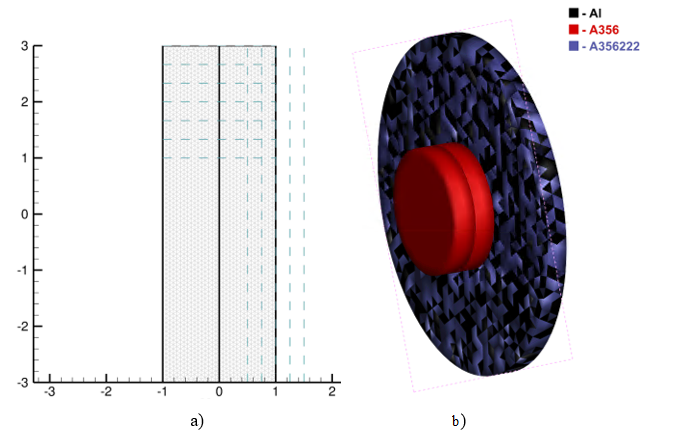
Figure 4 – Visualization of the location of fixed rays (planes) eray on geometry: a) 2D; b) 3D

Figure 4a shows an example of visualizing the location of multiple rays., on a 2D geometry file, after applying the eray directive. The dashed lines show the location of the two sets of fixed rays and the direction their actions. Figure 4b shows an example of visualizing the location of a plane on a 3D geometry file.

The result of the directive is a graph with averaged flow parameters. passing through the ray (plane) defined using this directive. In this case, averaging can be observed separately for destroyed particles moving through the beam, as well as for non-destroyed elements.

The discretization of parameter changes over time is determined by the directive print_at_every_step, and the monitored values are set by the directive printspy.

eray_mat is a directive that defines which materials must be taken into account to calculate the average in the directive eray. Thus , using this directive, it is possible to selectively calculate parameters. according to individual materials. By default, eray_mat=0 (all materials, involved in the calculation).

eray_body is a directive that defines which bodies must be taken into account to calculate the average in the directive eray. Thus , using this directive, it is possible to selectively calculate parameters. for individual bodies, for example, to estimate the speed of only the penetrating impactor into the barrier, without taking into account the target. By default, eray_body=0 (all bodies, involved in the calculation).

fracture_model = (ball|mball|cball|erosion|erosion_mass) a directive that defines the replacement model for destroyed elements in the calculation.

During high-speed impact, materials experience significant deformations., this is reflected in numerical methods or by the strong distortion of Lagrange cells. The way out of this situation is hybrid methods, where for areas of Grid methods are used with small or moderate deformations, and grid–free methods are used in areas with severe distortions [13-15]. The task of modeling the destroyed material by discrete particles of finite size includes two aspects: 1) replacing a solid damaged material with a discrete analog having the same parameters, i.e. mass, momentum and energy; 2) determination of the motion of discrete particles and their interaction with boundaries solid material, as well as between each other.

The following values are known in each cell of the difference grid: current density of the material, tensors of stresses and strain rates, specific internal energy. The velocity coordinates are assigned to the nodes of the difference grid. The calculation algorithm is implemented in such a way that if at least one of the destruction criteria is met in a cell of the calculation grid, then this cell is marked like a damaged one. The damaged condition is characterized by the fact that the material it resists only volumetric compression. A special case of this The material may be a medium in which the equation of state remains the same, but the shift modulus is zero. The loosening parameter characterizes the ability of the damaged medium to remain continuous under volumetric stretching. If then the medium is considered completely destroyed and the pressure in it is zero.

Further, if the cell with a sign of damaged material is located on When the loosening reaches the critical boundary of the calculated area, the material of this cell is replaced by a discrete particle, the radius of which is calculated. from the condition of fitting one particle into a triangular cell. In one step In terms of time, only one layer of boundary cells can be transformed into discrete particles, since it is assumed that the velocity of the fracture wave front does not exceed the velocity of propagation of the disturbance in the medium. Thus, the application of this calculation algorithm can in certain cases lead to the replacement of all cells of the computational domain with discrete particles, i.e. the transformation of a solid body into a cloud of particles.

Let the body contain a number of damaged cells, which are highlighted in Figure 5a. green and red colors. We present an algorithm for replacing cells containing damaged material when it reaches critical values with discrete particles of finite size that simulate the destroyed material.

The replacement algorithm is as follows (see Figures 5a and 5b):

• deleting the from the calculated mesh;

• replacing the triangular element with a discrete particle with the center and radius of the inscribed circle;

• all variables related to elements (mass, material, pressure etc.), are transmitted to a discrete particle;

• all the nodal characteristics of the element (speed, etc.) are transmitted a discrete particle from three nodes of the difference mesh based on the law of conservation of momentum;

• the mass of nodes, undisturbed neighboring elements, decreases by the mass of the nodes of the ;

• element transformations into a discrete particle is performed similarly as for the .

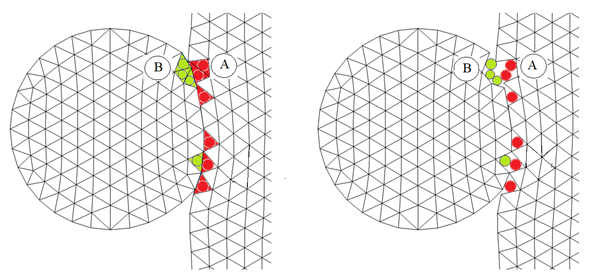
Figure 5 is an illustration of replacing destroyed cells with discrete particles

After replacing the element with a discrete particle, the connection with the solid body is broken and the discrete particle of finite size moves independently. A discrete particle with kinetic energy interacts with both a solid body and other discrete particles at the next time step , i.e. a hybrid approach of grid and grid-free algorithms is implemented.

A directive can take one of three values:

ball – the destroyed element is replaced by an incompressible particle in the shape of a circle or sphere in 2D or 3D, respectively, see Figure 6 (value by default);

mball – the destroyed element is replaced by several incompressible ones particles – four in 2D and six in 3D;

cball – destroyed elements are replaced by shrinking circles, implemented only in a 2D setting;

erosion – the destroyed element is removed along with the mass. This is a classic algorithm by M. Wilkins [16] with loss of system momentum;

erosion_mass – the destroyed element is removed and its mass is transferred into neighboring elements.

The algorithms erosion and erosion_mass are recommended to be used only to speed up the counting time, as a preliminary. Savings the counting time can reach up to 30%.

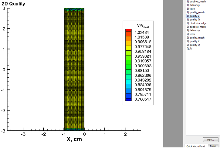
Figure 6 – Visualization of the directive's operation gdebug

gdebug is a directive that enables the output of debugging information when creating a geometry. Each step is displayed when working with the geometry. in the visualization program, for each body individually. The directive is necessary for developers, to find errors when creating geometries. In the picture 6 shows an example of how the directive works – the quality of the deviation of the difference grid from a perfect triangle. The sequence of creation is clearly shown geometry and its result at each stage of the software package execution.

geom_file is a directive that defines the name of the file in which the geometry of the problem will be written in the format necessary for visualization. The file is created in the work_dir directory.

geomonly is a directive that requires calculating only geometry and stop. If the task preprocessor detects such a directive in the configuration file, the task stops immediately after calculating the geometry of all objects. This option is useful when creating complex geometric objects., since it is often difficult to create the required geometric shape the first time. configuration, especially with an abundance of geometric conjugates.

ghost_time(ghost_start,ghost_stop) the directive that creates The ghost body. The ghost body is a computational area that can be “connected” and “disconnect” during the calculation process, as shown in Figures 7 and 8. The parameters of this directive include:

ghost_start – the time of the “appearance” of the ghost body in the counting process [msec];

ghost_stop is the time for the ghost body to “disappear” from the count [msec]. That is, this directive creates similar bodies with a specified lifetime. This directive can be used in a simplified form: ghost_time(ghost_start) when there is no need to exclude the body from the account.

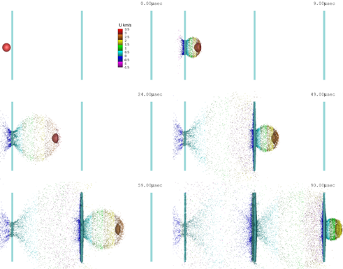
Figure 7 – Sequential penetration of a spaced barrier with calculation of all plates

The application of the directive makes it possible to significantly reduce the estimated time of such tasks, and to prevent the “collapse” of the solution with a huge number of estimated steps when rounding errors accumulate.

The default value is noghost, a directive that requires Don't create ghost bodies.

gmsh is a directive that defines the path to a binary file. gmsh programs. To use this command on your hardware, you must the corresponding program must be pre-installed (project page http://gmsh.info /).

gpu is a directive that forces the use of existing graphics card power to perform geometry calculations, nogpu is a directive that forces the program does not perform calculations on the GPU.

gpu_device is a directive that forcibly sets the number GPU devices(supported GPU devices can be found by running the HSDF MODULE program with the key “--gpuprint”).

The default device is gpu_device = 0.

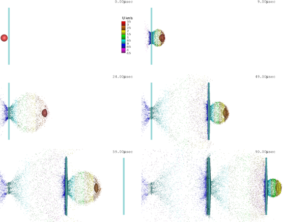
Figure 8 – Calculation results with sequential connection of plates in a spaced barrier using the ghost_time directive

hardwall is a directive that determines the presence of a hard wall in the task. All contact boundaries, including newly created ones as a result destruction is detected automatically. The hardwall directive specifies the fact that a boundary condition is used in the calculation is absolutely rigid. the wall. The rigid wall coordinate is set automatically, in parallel one of the axes, based on the initial kinematic conditions of the problem.

hardwall3 is a directive that defines the presence of three hardwalls the walls around the perimeter of the geometric object (glass). This option is necessary to emulate a plane shock wave in 2D problems.

knot_axial is a directive that defines the weight ratio for specifying the masses of nodes in a triangular cell in an axial 2D problem. (i is an integer >0). This option is intended for developers.

By default is knot_axial = 108. All other values can be output by setting a value that is obviously not incorrect, for example, knot_axial = 0.

lray is a directive that establishes a line of “sensors” for 2D tasks, or a plane of “sensors” for 3D that move together with the body and tracks the change of values in the cells over time, in the statement Lagrange. The directive is useful for averaging values in plane shock waves in heterogeneous media. The directive uses the following parameters:

lray(nx,dx);

lray(nx,dx,wl);

lray(nx,dx,wl,nl).

nx – defines the coordinate axis perpendicular to which the ray is directed. It is specified either as an integer from 1 to 3, or as an alphabetic expression., for example, X, Y or Z;

dx – defines the values of the nx ray coordinate, for example X=0.4;

wl – width of the viewing area, (default value 0 [cm]);

nl is the number of fixed rays in the viewing area (value by default, 1[pcs]).

The result of the directive is a graph with averaged parameters for all installed “sensors” defined using this directive. The discretization of parameter changes over time is determined by the directive print_at_every_step, and the monitored values are set by the directive printspy.

lsdyna is a directive that creates a k-file with a geometry for subsequent export to LS-DYNA.

By default, the file is not created.

mix_default a directive that sets default values for all mixtures involved in the task.

mix_default(hetero);

mix_default (hetero, maxelem);

mix_default (hetero, maxelem, allow_con);

mix_default (hetero, maxelem, allow_con, xmin, xmax);

mix_default (hetero, maxelem, allow_con, xmin, xmax, direct).

hetero is a type of heterogeneous material creation, one of the existing values (single|elem|knot|snake|paw|tie), geometric interpretation The types are shown in Figure 9;

knot – clustered (volumetric) foreign inclusions combined in the neighborhood of all the nodes of the element, based on a probability distribution, according to a given concentration (Figure 9a);

elem – clustered (volumetric) foreign inclusions combined in the neighborhood of all the faces of the element, based on a probability distribution, according to a given concentration (Figure 9b);

single – single inclusions of foreign material based on probabilistic normal distribution, according to a given concentration (Figure 9b);

snake – clustered foreign inclusions united in the neighborhood one of the facets of the element, based on a probability distribution, according to a given concentration (Figure 9d);

paw – cluster foreign inclusions united by a nodal the neighborhood of elements, based on a probability distribution, according to a given concentration (Figure 9e);

tie – clustered foreign inclusions united in the neighborhood one of the element nodes, based on a probability distribution, according to a given concentration (Figure 9g).

maxelem – the maximum number of elements in one heterocluster (by default: it is determined by the type of heterogeneous material creation);

You can also specify not only the type of inclusions in a heterogeneous matrix, but also the size of these inclusions. For example, Figure 10 shows the geometric configurations of a heterogeneous material with the same volume concentration (40% ceramics in a metal matrix), but different sizes of inclusions.

allow_con – determines whether previous hetero-inclusions should be taken into account when creating a material ([1] – take into account (default value), [0] – ignore);

xmin, xmax – defines the range of coordinates where it is necessary to determine "mix" (default: start and end of body);

direct – defines the direction of the layers and can be set as number or name ([1] – X (default), [2] – Y, [3] – Z).

netgen is a directive that defines the path to the binary file of the netgen executive program. To use this command on your The corresponding program must be pre-installed on the equipment (page the project https://ngsolve.org ).

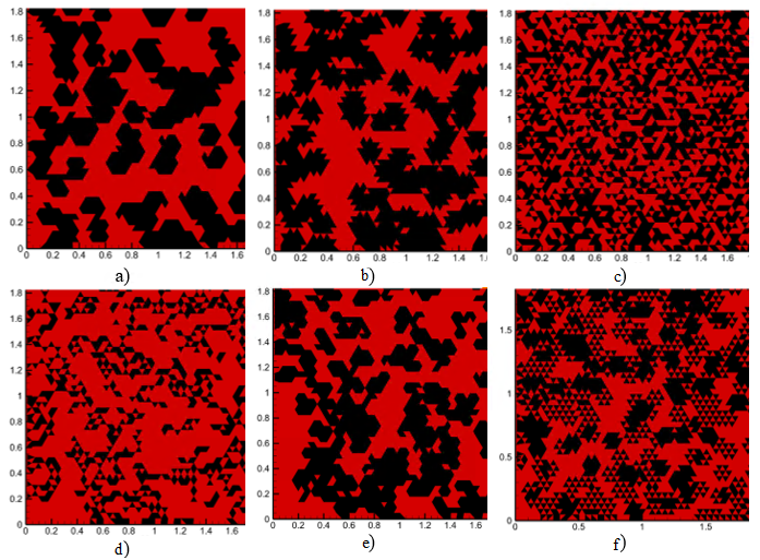
Figure 9 – Visualization of the directive's operation mix_default for heterogeneous inclusions of two materials:

a) – knot, b) – elem, c) – single, d) – tie, e) – snake, f) – paw

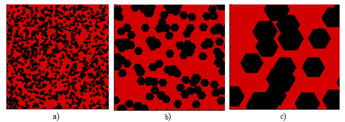
Figure 10 – Visualization of the directive's operation mix_default  for heterogeneous inclusions is the knot type made of two materials. Heterogeneous material with different maxelem size of inclusions:

a) 10 cells; b) 100 cells; c) 700 cells

nodump is a directive that determines that under no circumstances do not create intermediate dump files during the billing process.

num_dump is a directive that defines the maximum amount storing dump files simultaneously. During the billing process, intermediate files are created, the size of which can reach tens of gigabytes. However, the number of files stored at the same time is limited by the num_dump directive. As soon as the number of temporary storage files reaches the value num_dump, the software package starts rotating them in the DVR mode.

The default value is num_dump, depending on the total number of calculation files. (one order of magnitude less).

paraview is a directive that defines the path to the binary file of the executive program ParaView. To use this directive The appropriate program must be pre-installed on your hardware. (project page https://www.paraview.org /).

pie is a directive that allows the calculation of a quarter or half of the 3D geometry, as shown in Figure 11. The following parameters are used as variables:

pie(pie_vertex, pie_vector, r, h, angel);

pie(pie_vector, r, h, angel);

pie(r, h, angel);

pie_vertex is the origin of the coordinate of the cylinder (which cuts off the entire geometry tasks) covering the entire task ( by default 0,0,0);

pie_vector – the guide vector of the cylinder (default is 1,0,0);

r,h – radius and length of the cylinder;

angel – the counterclockwise angle to be cut off (180 to 360 degrees).

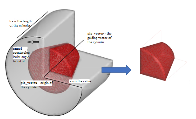
Figure 11 – how the pie directive works

Limitation: The directive can only be applied for axisymmetric geometry only when using gmsh and salome.

Example

pie(-1, 0, 0, 1, 0, 0, 400.0, 200.0, 270)

The result is shown for two angles of 180 and 270 degrees in Figure 12.

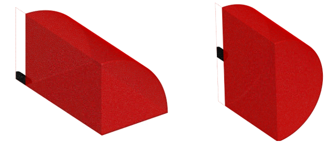
Figure 12 – The result of the directive pie:

a) angel =270 degrees; b) angel=180 degrees

ppp = (auto|paraview) a directive that defines an external program for post-processing (Post Processing Program). Each external program It has its advantages and disadvantages, and, therefore, the opportunity has been realized. define this program for a specific task. . The directive can accept one of the values is:

auto – defined through the specified variable calc_file;

paraview – sets as post-processing software: ParaView.

To automatically start the postprocessor at the end of the calculation, it is necessary defining paths to external programs in the configuration file.

By default – ppp = auto

print is a directive that describes the values of which values it must be saved in calculation files. Since the number of calculation files is it can reach several thousand, and the size of each file can reach tens of gigabytes, then to reduce the amount of information stored on the disk , the software package implements controlled output of variables to a file. the calculation, which is determined using the print directive, according to the notation given in Table 1.

If you add a “–” (minus) sign before any designation, then disable it. output of a specific variable. The values of coordinates and velocity vectors are saved always.

By default, output only pressure and pulse print(p,i).

Table 1 – Options for the print

directive

printspy – describes which values to store in cells with sensors. Since there is no need to keep the same values as for both in the calculation and in the sensors, the directive allows you to differentiate the output of the values for calculation and in installed sensors. For example, the calculation requires artificial viscosity output, but this parameter does not need to be output in sensors. The designations of the values are similar to those shown in Table 3. Regardless of the specified directive, the values of coordinates, velocity vector and pressure they are always saved.

printspy(all) – saves all possible values.

By default, it copies values from the print directive.

print_at_every_step is the directive that performs the recording momentum, speeds, and other parameters set for tracking nodes and/or elements at each time step. The result of the directive shown in Figure 13. The picture shows the smoothness of the lines when applied this directive. In addition, if it is necessary to monitor the “Strength” parameter, then it is necessary to include this directive, since the force is determined through the derivatives obtained as a result of the calculation. Using this option significantly increases the calculation time, since the disk write operation is quite slow. So the calculation time in Figure 13a is 15 seconds, and the time The calculation shown in Figure 13b takes 32 seconds.

By default - noprint_at_every_step, recording is performed together with the calculation record defined by the time directive.

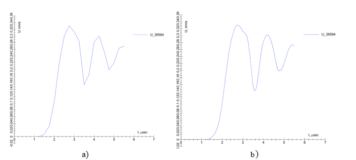
Figure 13 – The result of the work:

a) – noprint_at_every_step; b) – print_at_every_step

protect is a directive that allows you to protect the directory with the calculation files from being overwritten with a new calculation when working in the same directory. The software package will refuse to record a new calculation to a secure directory by offering to change it to another one.

By default is noprotect, the directory is not protected from overwriting.

randlaw = (uniform|gauss|weibull|binomial|gamma|chisq|exp|poisson|power|beta|nbinomial|wigner) – The directive describes the law according to which the random variable will be distributed when the random number generator is running, as when creating heterogeneous materials, as well as when creating the initial properties of the material “as part of the delivery.”

Learn more about the laws of distribution:

1) uniform is a continuous uniform distribution, shown in Figure 14a is the distribution of a random real quantity taking values belonging to a certain interval of finite length, characterized by by the fact that the probability density in this interval is almost constant everywhere (https://en.wikipedia.org/wiki/Continuous_uniform_distribution).

2) gauss is the Gaussian distribution shown in Figure 14b. The normal distribution, also called the Gaussian distribution, is a distribution the probability distribution, which in the one-dimensional case is given by a probability density function that coincides with the Gaussian function (https://en.wikipedia.org/wiki/Normal_distribution ).

3) weibull – The Weibull distribution is a two-parameter family of continuous distributions shown in Figure 14b. Named after Waloddy Weibull, who described it in detail in 1951, although for the first time it was identified by Frechet in 1927 (https://en.wikipedia.org/wiki/Weibull_distribution ).

4) binomial is the binomial distribution shown in Figure 14g, which is the distribution of the number of "successes" in a sequence of n independent random experiments such that the probability of "success" in each of them is constant and equal to p (https://en.wikipedia.org/wiki/Binomial_distribution ).

5) gamma is the Gamma distribution shown in Figure 14d, which is a two-parameter family of absolutely continuous distributions (https://en.wikipedia.org/wiki/Gamma_distribution ).

6) chisq – Chi-square test – any statistical test hypotheses in which the sample distribution of the criterion has a distribution chi-squared, provided that the null hypothesis is true, is shown in Figure 14e. It is believed that the chi-square criterion is a criterion that is asymptotically is correct, that is, the sample distribution can be made as close as possible to the chi-square distribution by increasing the sample size (https://en.wikipedia.org/wiki/Chi-squared_test ).

7) exp is the exponential distribution shown in Figure 14j, an absolutely continuous distribution that simulates the time between two successive occurrences of the same event (https://en.wikipedia.org/wiki/Exponential_distribution ).

8) poisson is the Poisson distribution shown in Figure 14z, This is a distribution of a discrete type of random variable, which is the number of events that occurred in a fixed time, provided, that these events occur with some fixed average intensity and independently of each other (https://en.wikipedia.org/wiki/Poisson_distribution ).

9) power is a functional relationship between two quantities in which a relative change in one quantity leads to a proportional relative change of another value, regardless of the initial values of these quantities: the dependence of one quantity on another is a power function (https://en.wikipedia.org/wiki/Power_law ).

10) beta – In Bayesian inference, the beta distribution shown in Figure 30k, is the conjugate a priori probability distribution for Bernoulli distributions, binomial, negative binomial, and geometric distributions. The beta distribution is a suitable model for the random behavior of percentages and proportions (https://en.wikipedia.org/wiki/Beta_distribution ).

11) nbinomial is a negative binomial distribution, also called the Pascal distribution, shown in Figure 30L, is the distribution a discrete random variable equal to the number of failures in a sequence of Bernoulli trials with a probability of success p, conducted before the rth success (https://en.wikipedia.org/wiki/Negative_binomial_distribution).

12) wigner – Semicircular law (or distribution) Wigner's ring, shown in Figure 30m, is named after physicist Eugene Wigner. a continuous probability distribution on a straight line whose density graph it is obtained after normalization from a semicircle constructed on the segment [-R, R] as on the diameter (https://en.wikipedia.org/wiki/Wigner_semicircle_distribution ).

By default is randlaw = uniform.

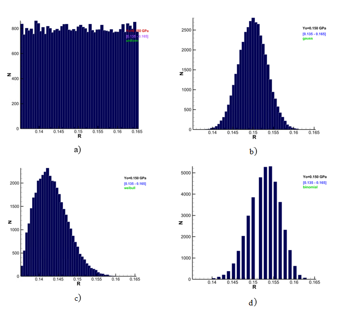
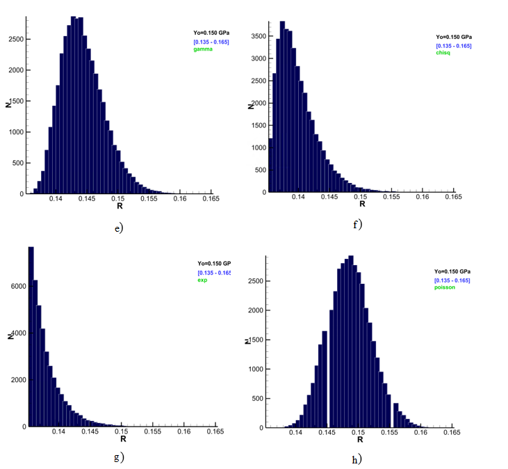
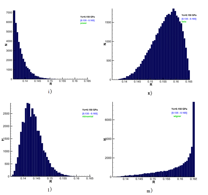
Figure 14 – Distribution of yield strength in a material according to the law:

a) Uniform distribution; b) Gaussian; c) Weibullian d) binomial;

e) gamma; f) with chi-square criterion; g) exponential; h) Poisson;

i) power-law; k) beta; l) negative binomial; m) Wigner

refine_mesh is a directive that requires improving the quality of the created or imported mesh. The use of the dynamic method implemented in the software package significantly increases the number of high-quality triangular cells, while cells with low quality “disappear”, as their quality increases in the process of dynamic correction. The application of local grid restructuring, after dynamic impact, significantly corrects triangles with low quality.

refine_quality – sets the minimum value of the grid quality, to which the software package tries to improve the quality of individual cells grids. The value of the quality criterion is the normalized value of Q and is in the range Q ∈ (0, 1], with the value Q=1 corresponding to the correct a triangle or tetrahedron, and Q=0 corresponds to a degraded triangle or a tetrahedron, in 2D and 3D respectively. Possible range of quality settings grids 0.5 – 1. The higher the value of this parameter, the more time is needed to implement this condition.

By default – refine_quality = 0.75.

remove_bad_elem is a directive that declares to forcibly destroy low–quality items that define a “time step" in the billing process. noremove_bad_elem is a directive that prohibits the forced destruction of bad elements that define a “time step" in the billing process.

By default is remove_bad_elem.

restart – "to the invoice". The “restart” directive instructs the program resume the calculation using the dump file as the initial data.

run_paraview– the directive determines that at the end of the calculation you need to run the visualization program ParaView, depending on how the ppp directive is defined. Directives norun_paraview they determine that there is no need to start automatically at the end of the calculation. an external post-processing program (default value).

qhull is a directive that defines the path to the binary file of the Qhull execution program. To use this command on your the corresponding program must be pre-installed on the equipment (https://www.qhull.org ).

safe is a directive that launches a secure algorithm for calculating contact boundaries (slow). The program code uses different methods the search for new contacts and powers gained as a result of the destruction of the multitude objects. By default, the code uses a “windowed” search method., as the fastest. In 90-95% of the calculations carried out by us – this search most justified. There is also a secure search embedded in the program code, which, true, it searches for contacts, but it significantly increases the calculation time. And if you find border crossings during the calculation process, then stop the program and use the safe directive to enable safe mode., which will help to overcome the difficulties that have arisen.

sensor_elem, sensor_knot – directives that set the “sensor" in the node and/or element according to the specified coordinates. The sensor is needed to track time-related changes in parameters such as speed, pressure, voltage , etc . The CAE Fidesys software package with the HSDF module implements There are several ways to specify the installation of sensors in the calculation model.

You can install “sensors” using the directives 1) spy_knot, spy_elem explicitly specifying the element and/or node number, which minimizes the error of installing “sensors”, but is rigidly tied to geometry and pitch; 2) sensor_knot, sensor_elem explicitly specifying the installation location by coordinates, which allows you to ignore the specified step of the geometry and the order of its construction; 3)sensor_line defining a plane for installing multiple “sensors” to calculate the average value of quantities, usually for heterogeneous materials. The discretization of parameter changes over time is determined by the print_at_every_step directive, and the monitored values are set the printspy directive. If the element and/or node are in the calculation process if it collapses, then its values are reset to zero.

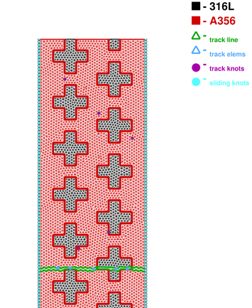
Figure 15 – Geometric model with installed "sensors" using directives sensor, spy or ray

Figure 15 shows an example of a geometric model with "sensors" installed using various directives sensor or spy. With the help of color differentiation, it is possible to control the correct installation of the sensors indicated in the legend, so that the monitored nodes are marked with purple circles, and the elements – blue triangles, etc.

The sensor_knot, sensor_elem directives use the following parameters:

sensor_elem(x, y, z) – tracking values in a triangular element the grid, the coordinates (x,y,z) of which is located inside;

sensor_knot(x, y, z) – tracking values at the nearest node a grid that is located in the area indicated by the coordinates (x,y,z).

Figure 16 shows an example of visualizing the pressure value over time using five specified elements. In the legend, the number is the element number. Automatically, with the help of a thick black line, the average value is calculated for all the specified “sensors".

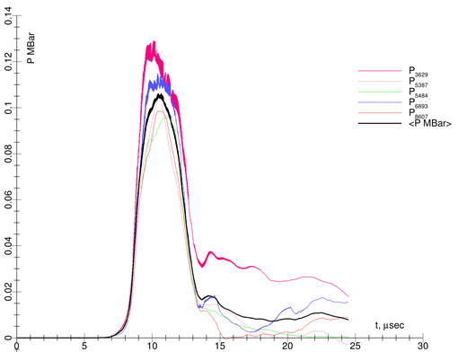
Figure 16 – Pressure output result in the elements using the sensor_elem directive

spy_knot, spy_elem is a directive that installs a “sensor” in a node or element according to the specified element numbers and/or nodes, respectively. The directives are completely similar to sensor_elem and sensor_knot, only with explicit numbers.

spy_elem(num1, num2,...) – tracking parameters in a triangular grid element with numbers num1, num2, etc.;

spy_knot(num1, num2,...) – tracking parameters in a grid node with numbers num1, num2, etc.

step is a directive that defines a step in space [see]. The pitch is set to be the same for all geometric primitives, using which represent the geometric model of the problem.

The maximum value of the space step that can be calculated is limited only by the geometric dimensions of the objects. If the value is still selected above the maximum allowed value for at least one of the geometric primitives, the program is forcibly stopped, and the output recommendations for changing the step. Minimum step value in the software the complex is not limited, but as practice shows, the use of a step is less 0.001 cm leads to errors in calculations related to loss of accuracy when calculations of differential equations on a triangular grid and machine rounding, with a large number of time steps.

The directive must be specified, and there is no default value.

storage = (binary,zlib,bzip2) is a directive that defines the file format for storing the internal files of the program. When the software is running The module creates a lot of internal files that may be in demand. for subsequent calculations, for example, the geometry of objects with a created grid, dump files, fragment files, etc. So the size of temporary files is With three-dimensional calculations, it can reach several gigabytes, so to minimize disk space, there is a directive governing the storage format. these files. This directive can take one of the values:

binary – binary compression is used. Data compression and decompression from the hard disk is carried out as quickly as possible and is limited only to the parameters of the hard disk. The size of the created files is the largest of all available compression methods (default value).

zlib is a free cross-platform library used for zlib data compression, which provides in-memory compression and decompression functions, including checking the integrity of uncompressed data. The size of the files being created is about 2 times smaller than using the binary compression method, but additionally leads to an increase in the time required for calculation. the CAE Fidesys software package with the HSDF module.

bzip2 – a free cross-platform library is used for bzip2 data compression [17], which provides compression functions and in-memory decompression, including checking the integrity of uncompressed data. The size of the files being created is the smallest of all the compression methods available, but additionally leads to an increase in the counting time required. for the CAE Fidesys software package with the HSDF module.

tetgen is a directive that defines the path to the binary file of the Tetgen executive program. To use this directive on your The corresponding program must be pre-installed on the equipment (page the project http://wias-berlin.de/software/index .jsp?id=TetGen).

time is a directive that sets the duration of the numerical an experiment.

time(t_end, t_print), set in [microseconds]. The directive must be specified .

t_end - the time after which the task stops;

t_print is the period for recording intermediate calculation results in a file.

These parameters can be set together using the time directive., This can be done separately using the t_end and t_print directives. In the latter case, setting the t_print directive is not a prerequisite, and the recording period is calculated based on 1/10 t_end.

triangle is a directive that defines the path to the binary file of the Triangle execution program. To use this command on your The corresponding program must be pre-installed on the workstation. (program website https://www.cs.cmu.edu /~quake/triangle.html ).

type_calc = (axial|plain|calc3d) – a directive that defines the type of task. The directive must be specified , the default value is absent. The task type can take one of three values:

axial – calculation in 2D axial symmetry. The axis of axial symmetry runs along the OY axis in Cartesian coordinates;

plane – calculation of a flat 2D problem;

calc3d – 3D calculation.

All directives can be specified using type_calc =..., or separately: axial, plane, calc3d.

viscosity is a directive that defines the parameters of artificial the viscosity of the difference scheme. The directive uses the following variables:

viscosity (cl, cq, dt)

cl – coefficient for linear viscosity, range [0.10);

cq is the coefficient for quadratic viscosity, range [0.10);

dt is the time margin coefficient, range (1e-3.0.33).

These parameters can be set together using the viscosity directive., and separately using the directives coef_cl, coef_cq, coef_dt. It is not recommended to change these parameters, they are primarily intended for for developers. The current value of all parameters can be viewed by running calculation with the option to output debugging information.

By default is viscosity (1.0, 4.0, 0.25).

xray is a directive that defines the installation location multi-frame recording of fast-moving processes using Synchrotron radiation (SI). The Directive uses the following variables:

xray(nx,dx);

xray(nx,dx,wl);

xray(nx,dx,wl,nl).

nx – defines the coordinate axis perpendicular to which it is directed the beam of light. It is indicated either as an integer from 1 to 3, or as a letter expression, for example X, Y or Z;

dx – defines the values of the nx ray coordinate, for example X=0.4;

wl – wiggler width, (default value is 2 [cm]);

nl is the number of SI rays (the default value is 512 [pcs]).

Figure 17 shows an example of visualizing the location of a wiggler on a geometry file after applying the xray directive. Yellow lines The size and location of the wiggler are shown. Wiggler (from the English wiggle — wiggle, bend) is a device for generating synchrotron radiation in an electronic a synchrotron storage device.

The result of the macro is presented in the last section on the postprocessor.

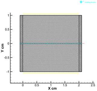
Figure 17 – Visualization of the wiggler location on geometry when applying the xray directive

warn2err is a directive that can be used to translate a part of warnings issued by the software are classified as “error”, i.e. the program is completely stopped until the cause that caused this error is eliminated. It is useful when debugging the properties of materials for outdated parameters , etc.

By default is nowarn2err.

work_dir is a directive that defines the path to the working directory where all calculation files of the current project will be stored. You can set both the absolute path and the relative path from the configuration file.

If another project is found in this folder, then all the files of the previous one calculations are deleted without warning.

Literature

1. Sutherland I.E., Hodgman G.W. Reentrant polygon clipping // Commun. ACM. 1974. Vol. 17, № 1. P. 32–42.

2. Kraus E.I., Shabalin I.I., Shabalin T.I. Automatic tetrahedral mesh generation for impact computations // AIP Conference Proceedings. 2017. Vol. 1893. P. 030129.

3. Andreev A.N., Kraus E.I., Shabalin I.I. etc. Mechanics - from discrete to the continuous one. -Novosibirsk: Publishing house of the SB RAS, 2008. -344 p. Novosibirsk: Publishing house SB RAS, 2008. 344 p.

4. Kraus E.I., Fomin V.M., Shabalin I.I. Simulation of the collision process complex two-dimensional bodies against a deformable obstacle // Computational technologies. 2006. Vol. 11. P. 104–107.

5. Kraus E.I., Kraus A.E., Shabalin I.I. The Influence of the Contact Boundary in a Metal Matrix Composite on Dynamic Loading // Springer Proceedings in Physics. 2024. Vol. 1067 SPPHY, № November. P. 134–142.

6. Kraus E.I., Fomin V.M., Shabalin I.I. Dynamic construction method triangular meshes in multiply connected areas // Computational technologies. 2009. Vol. 14, No. 5. P. 40–48.

7. Shimada K., Gossard D.C. Bubble mesh // Proceedings of the third ACM symposium on Solid modeling and applications - SMA ’95. New York, USA: ACM Press, 1995. P. 409–419.

8. Conway J.H., Torquato S. Packing, tiling, and covering with tetrahedra // Proc. Natl. Acad. Sci. 2006. Vol. 103, № 28. P. 10612–10617.

9. Joe B. Geompack — a software package for the generation of meshes using geometric algorithms // Adv. Eng. Softw. Work. Elsevier, 1991. Vol. 13, № 5–6. P. 325–331.

10. Barber C.B., Dobkin D.P., Huhdanpaa H. The quickhull algorithm for convex hulls // ACM Trans. Math. Softw. 1996. Vol. 22, № 4. P. 469–483.

11. Si H. TetGen, a Delaunay-Based Quality Tetrahedral Mesh Generator // ACM Trans. Math. Softw. 2015. Vol. 41, № 2. P. 1–36.

12. Shewchuk J.R. Triangle: Engineering a 2D quality mesh generator and Delaunay triangulator. 1996. P. 203–222.

13. Johnson G.R., Beissel S.R., Gerlach C.A. A 3D combined particle-element method for intense impulsive loading computations involving severe distortions // Int. J. Impact Eng. Pergamon, 2015. Vol. 84. P. 171–180.

14. Kraus E.I., Shabalin I.I. Reactor2D: A tool for simulation of shock deformation // AIP Conf. Proc. 2016. Vol. 1770. P. 030092.

15. Petrov I.B. et al. About the combined method for numerical solution dynamic spatial elastoplastic problems // Academy Reports Sci. 2015. Vol. 460, No. 4. P. 389–391.

16. Wilkins M.L. Calculation of elastoplastic flows // Computational methods in hydrodynamics / ed. Older B., Fernbach S., Rotenberg M. Moscow: World, 1967. P. 212–263.

17. Official website of the bzip2 library.

18. Kraus A. et al. Numerical Modelling of High-Speed Loading of Periodic Interpenetrating Heterogeneous Media with Adapted Mesostructure // Appl. Sci. 2023. Vol. 13, № 12. P. 7187.

19. Tables of physical quantities. Directory. /ed. Kikoina acad. I.K. Moscow: Atomizdat, 1976. 1008 p.

20. Kraus E.I., Fomin V.M., Shabalin I.I. Model thermodynamic equations functions of the state of substances. 2. Liquid and description of melting // Physical mesomechanics. 2004. Vol. 7. P. 289–292.

21. Fomin V.M., Kraus E.I., Shabalin I.I. A few-parameter equation of state of the condensed matter and its application to the impact problems // EPJ Web Conf. 2010. Vol. 10. P. 00027.

22. Fomin V.M., Kraus E.I., Shabalin I.I. An equation of state for condensed matter behind intense shockwaves // Mater. Phys. Mech. 2004. Vol. 7, № 1. P. 23–28.

23. Kraus E.I. Few-parameter equation of state of a solid at high energy densities // Bulletin of NSU. 2007. Vol. 2, No. 2. P. 65–73.

24. Kraus E.I., Shabalin I.I. A few-parameter equation of state of the condensed matter // J. Phys. Conf. Ser. 2016. Vol. 774. P. 012009.

25. Kraus E.I., Shabalin I.I. Calculation of elastic modules behind strong shock wave // J. Phys. Conf. Ser. 2015. Vol. 653. P. 012085.

26. Kraus E.I., Shabalin I.I. A new model to determine the shear modulus and Poisson’s ratio of shock-compressed metals up to the melting point // High Press. Res. 2021. Vol. 41, № 4. P. 353–365.

27. Marsh S.P. LASL Shock Hugoniot Data // Los Alamos Series on Dynamic Material Properties. Univ of California Press, 1980. 150 p.

28. Trunin R.F. et al. Experimental data on shock wave compression and adiabatic expansion of condensed matter / ed. Trunina R.F. Sarov: RFNC-VNIIEF, 2006. 531 p.

29. Kinslow R., ed. High-velocity impact phenomena / ed. Nikolaevsky V.N. Moscow: Mir, 1973. 533 p.

30. Kraus E.I., Fomin V.M., Shabalin I.I. Accounting for electronic components in the equation of state when calculating shock waves in a mixture of metals // Vestnik Perm National Research Polytechnic University. Mechanics. 2001. No. 9. P. 78–84.

31. Kraus E.I., Shabalin I.I., Shabalin T.I. Numerical analysis of wave propagation in a cermet composite // AIP Conference Proceedings. 2017. Vol. 1893. P. 030130.

32. Fomin V.M. et al. Accounting for Functions of Distribution of Mechanical Properties of Metals in Dynamic Processes of Deformation and Destruction of Barriers // J. Eng. Phys. Thermophys. Springer, 2022. Vol. 95, № 7. P. 1–9.