Tracking the Process of Solving a Nonlinear Problem Based on Convergence.log

Let us consider the process of solving equations for nonlinear processes using the example static setting.

After standard finite element discretization of the equilibrium equation the task boils down to the following: find the vector of nodal displacements u _n+1, satisfying the equation: nonlinear processes using the example static setting.

where f ^int , f ^ext - vectors of internal and external forces at the nodes, respectively.

This equation is nonlinear. In CAE Fidesys it is solved using the Newton-Raphson iterative method. Each iteration of this method represents solution of linearized problem (1).

Let the approximation be known . Then iteration ( k ) of the Newton-Raphson method is reduced to a linear system of equations:

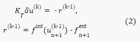
where r ^(k-1) , δu ^(k) - absolute force increments and displacements, respectively (in CAE Fidesys absolute residuals | r ^(k-1) | , | δu ^(k) | designated as ABS. FORCE RESIDUAL, ABS. VARIABLE RESIDUAL).

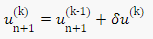
Having solved system (2), we update the nodal movements in the form:

The solution process by the Newton-Raphson method is illustrated using the figure:

The criteria for stopping the iterative process depend on the characteristics of the model.

Let's look at them in more detail.

Let us introduce the concept of relative residuals of forces and displacements, respectively:.

Their equivalents in CAE Fidesys are denoted as REL. FORCE RESIDUAL and REL. VARIABLE RESIDUAL.

Then the rationale for the conclusion about solution (2) and stopping the iterative process follows from the standard sentences:

relative residuals for two values (REL. FORCE RESIDUAL and REL. VARIABLE RESIDUAL) or residual ABS. VARIABLE RESIDUAL (for the case when the absolute increments of model displacements are close to the accuracy of mathematical calculations) became (became) less than the threshold;
relative residuals for one of the values (REL. FORCE RESIDUAL or REL. VARIABLE RESIDUAL) for the case of plasticity with contact in small deformations;
same as 1 or below the threshold, the discrepancy ABS decreased. FORCE RESIDUAL (for the case when the absolute increments of model forces are close to the accuracy of mathematical calculations).

This criterion is used for cases not presented in 1 and 2. In fact, we are talking about calculations with finite deformations, possibly going in conjunction with other nonlinearities.

Nonlinear calculation may end for the following reasons:

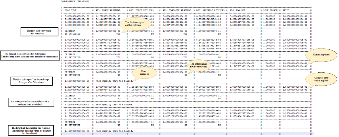
Convergence has been achieved according to one of the criteria depending on type of task. In the lineIS SATISFIED there will be one or more columns value YES;
The maximum number of iterations has been reached: “Maximum number of iterations has been reached";
One or more elements have lost stability due to large deformations“Mesh quality test has failed”.

In cases 2 and 3, a possible solution would be to increase the minimum number steps or maximum number of iterations. However, if the number of iterations more than 20, this means the convergence is very slow and it is advisable to check statement of the problem. You can also pay attention to cases where the residuals increase during iterations, usually this is a sign that the problem will not converge.

Substeps

Let us introduce the concept of substeps for a nonlinear problem. The convergence of the problem depends from the initial approximation, the further it is from the solution, the worse the convergence. To fix this you need to apply a smaller fraction of the load (column RATIO), to reduce displacement increments. To control data Several parameters are entered in substeps:

The initial number of substeps determines the length of the first substep;
The minimum number of substeps determines the maximum length substep;
The maximum number of substeps determines the minimum length substep;

If a substep converges, then the length of the next step will increase, until until it reaches 1/(number of minimum substeps).

If a substep diverges, it will be restarted with a zero initial approximation. Then, in case of failure, the length of the substep will be halved and decrease until it reaches the value 1/(number of maximum substeps). In this case, the calculation will fail.

Additionally, the length of the substep can be reduced in plastic problems, if plastic deformations exceed a certain threshold.

In static tasks, the LOAD TIME column indicates the current time. This time is conditional and equal to 1 for one static step. Column RATIO shows the proportion of applied loads of this static step.

For dynamic nonlinear problems, the algorithm for splitting steps is described above is also applicable, however in this type of calculation there are dynamic time steps replace the minimum number of steps, and setting the number of initial steps are ignored.

The LOAD TIME column indicates the current time, and the RATIO column shows the proportion of applied loads for a given step.

NOTES:

Threshold based on absolute values ABS. FORCE RESIDUAL, ABS. VARIABLE RESIDUAL is not directly specified by the user. It counts as 1e-8, multiplied by the user-specified relative accuracy;
The concepts of the threshold of absolute and relative residuals used are actually set by the user via the relative parameter accuracy. This accuracy is maintained by CAE Fidesys when There is no splitting of the substep when u _n+1 is found. Splitting a substep into several additional ones is used if the method Newton-Raphson does not converge at the initial substep. In this case the threshold adjusted automatically according to the degree of crushing.

The figure below shows an example of the contents of the Convergence.log file (for tasks with settings: 2 - static steps, minimum number of substeps - 2, maximum number of substeps - 8, maximum number of iterations - 10):