Search the documentation
Enter at least 2 characters
Enter at least 2 characters
 |
CAE Fidesys 9.0 Documentation |
The program Fidesys Viewer is used for visualization and analysis of the obtained results:
You don’t need to install FidesysViewer individually as it is included into the CAE Fidesys package. You don’t need a license to use FidesysViewer: the results of calculations obtained by using the CAE Fidesys preprocessor are available for viewing in FidesysViewer even after the license expires.
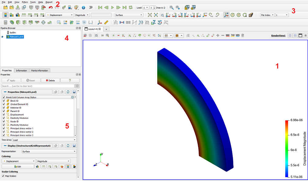
Workbench (1) displays the model and visual effects.
Main Menu (2) includes standard operations for working with files and projects, managing the visualization modes, panel display settings, filters, tools, and help available in the drop-down lists of the menu.
Toolbar (3) comprises the buttons for calling the most frequently used commands while working with the program.
Pipeline Browser (4) includes the opened models and filters applied to them.
Properties Page (5) displays the properties of the selected object in the Workbench or in the Pipeline Browser.
You can show or hide additional panels in the menu View.
Fidesys Viewer allows you to view and analyze the results. You can do that using multiple filters selected in the item View in the menu. Some of them are described below.
Fields and components of display can be selected in the Toolbar:

You can also see the Color Map by clicking  in the
Toolbar.
in the
Toolbar.
In order to select points or cells, use the following buttons in the Toolbar:

Numerical results for the data fields can be viewed in the tab Information. If the entire model is in focus, the fields of the tab Information contain a range of data – from minimum to maximum value.
The values in points can be found using the filter Probe Location (Filters
→ Alphabetical → Probe Location). Then you must specify the viewing
point coordinates. After applying the filter, data field values are displayed
only for the specified point in the tab Information.
 Detailed.
It is also possible to view the numerical results for the selected points by clicking Point Information on the Toolbar.
The values in the points/nodes/elements can be identified and viewed by using Selection Inspector (View → Selection Inspector).
To view the strained model, select Filters → Alphabetical →
Warp By Vector. In the Properties tab, you can select the display
scale.
To quickly access the filter, click Warp By Vector on the top panel. Detailed.
To receive data from the spherical or cylindrical coordinate systems, select Filters → Alphabetical → Coordinate systems. Next, select the data field that you want to represent in new coordinates. After applying the filter, a new data field will appear in the tab Information, for example, Stress (spher.).
To graph along a straight line, select Filters → Alphabetical → Graph along a straight line.
Specify coordinates of the beginning and end of the line. In the tab View, select the appropriate data field to display in the graph. Detailed.
To graph along a curve, select nodes (see par. Selection) for which graph will be plotted. Next, use Filters → Alphabetical → Extract selected and then Filters → Alphabetical → Show data. Detailed.
To plot a time dependency graph, you should allocate points of interest through the Allocation Inspector or by the button Select points in the standard string and then apply the filter Filters → Alphabetical → Plot selection over time.
To estimate the mesh quality, select View → Filters → Alphabetical → Mesh Quality. Specify the necessary settings in the tab Properties. After applying the filter, the new fields which analysis allows concluding about the mesh quality will appear in the tab Information.
To view the model slice, select Filters → Alphabetical → Slice. Specify the normal or the direction in which you want to make the slice. Detailed.
To view the model cross section, select Filters → Alphabetical → Cross section. Specify the normal or the direction in which you want to make the slice. Detailed.
 To view beams and shells in 3D in the FidesysViewer
postprocessor, you can click on the button 3D in the
standard string.
To view beams and shells in 3D in the FidesysViewer
postprocessor, you can click on the button 3D in the
standard string.
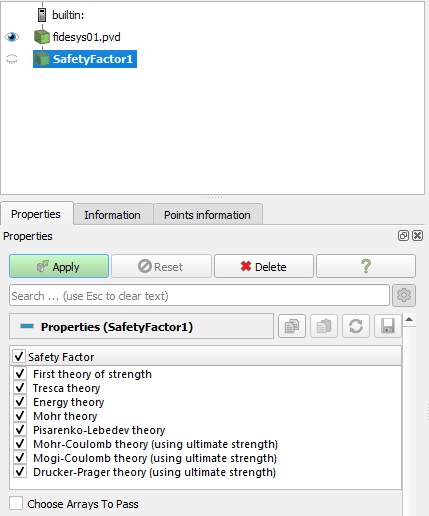
To view the model cross section, select Filters → Alphabetical → Safety Factor. If the ultimate strength and yield strength were not specified when preprocessing, you should set them in the tab Properties. Safety factor is calculated by the first theory of strength, energy theory, Tresca theory, Mohr’s theory of failure, Pisarenko-Lebedev theory. Obtained values can be viewed in the tab Information in the new field Safety Factor. The first component of the field is the safety factor by the first theory of strength; the second is the safety factor by the energy theory, etc.
Formulas for Strength Criteria
σt — uniaxial tensile strength;
σc — uniaxial compression strength;
σm — tension von Mises;
c — soil cohesion;
φ — angle of friction;
σ1 — first major stress;
σ2 — second major stress;
σ3 — third major stress;
n — the field of the safety factor that needs to be displayed.
1. Calculation according to the first theory of strength.
It is used in the assumption of brittle fracture. By contours σ1 contours of safety factors are built n = σt / σ1.
2. Calculation according to the energy theory of strength (Mises stress).
It is used in the assumption of viscous fracture or if plastic state is not allowed.
By contours σi isolines of safety factors are built n = σy / σm or n = σ0,2 / σm, where σy or σ0,2 – physical or conditional yield strength.
3. Calculation according to the Pisarenko-Lebedev theory.
It is used in mixed fracture.
By fields σm and σ1 contours of safety factors are built
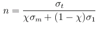
where 
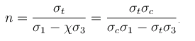
4. Calculation according to the Mohr’s theory, mixed destruction.
Contours of the safety factor
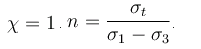
5. The third theory of strength by Tresk, viscous destruction or prevention of plastic flow.
A special case from Mohr's theory for
6. Mohr-Coulomb Criterion
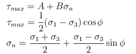
- normal stress on the fracture plane A = c; B = - tanφ or If strength limits are specified σc and σt, then
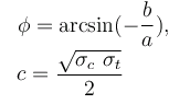
a = σt + σc; b = σt - σc < 0 (with b > 0 the angle of internal friction becomes negative, which is unacceptable)
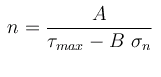
Safety factor:
7. Mogi-Coulomb Criterion
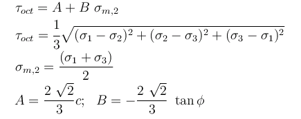
or

Safety factor
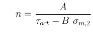
8. Drucker-Prager criterion
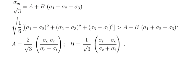
or
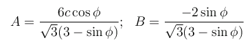
Safety factor:

This criterion was developed to describe the plastic deformation of clay soils. You can also use it to describe the destruction of rocky soils, concrete, polymers, foam and other pressure-dependent materials.
9. Navier criterion
Another name for the Mohr - Coulomb criterion
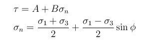 - the
normal stress at failure; A = c; B = - tanφ
- the
normal stress at failure; A = c; B = - tanφ
The minus is due to the fact that compression should lead to hardening, and compression σn corresponds to negative values c = - τB - tensile strength (shear), which is entered by the user for each material, or cohesion;

To plot the frequency dependencies after performing a calculation using harmonic analysis, select Filters → Index → Harmonic Analysis. Specify the node number, the characteristics of which will be presented on the graph.
To get numerical values of the obtained results, save the data in .csv format. Click Ctrl+S or select File → Save to do this. The saved file is an ordinary table of numerical data which can be opened in any text editor.
For dynamic problems, saving the model variation under deformation is available. To do it Select File → Save Animation.