CAE Fidesys 9.0 Documentation

Random Vibration

In mechanical engineering, random vibration is motion that is not deterministic, meaning that future behavior cannot be accurately predicted. Common examples include a car driving on a rough road or the load on an airplane wing during flight.

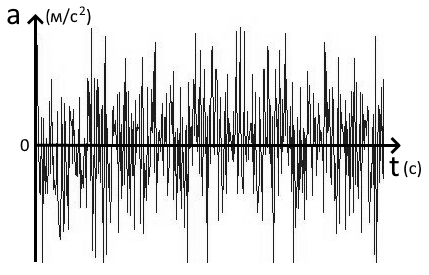
The response of a structure to random vibration is usually considered using statistical or probabilistic approaches. According to GOST 28223-89, there is a concept of "spectral density of acceleration" (SDA), expressed in units of "acceleration squared divided by frequency" ([(m/s^2)^2]/Hz). The term "power spectral density" (PSD) is more commonly used, but in the case of random vibration, the PSD and SPD are the same thing.

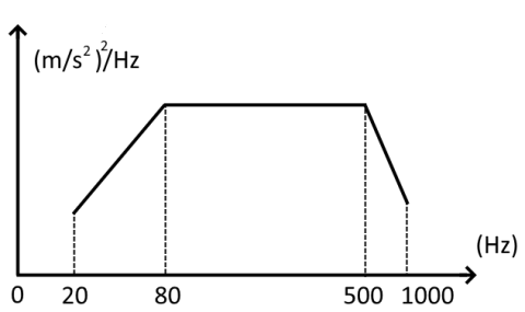
In considering time and harmonic analysis, we considered the disturbing forces as deterministic functions, i.e. changing with time or frequency according to a known law. In a large number of technical problems, external loads are random variables. When designing a structure, we have only statistical data on the winds in a given area. Important examples of response to random impacts are vibrations of transport vehicles caused by road irregularities; vibrations of structures caused by the pressure of a jet engine.

At the moment, the Fidesys software package implements an analysis of random vibrations with the following assumptions:

• the external random load is distributed according to the normal law of distribution of a random function

• the external random load contains the properties of stationarity and ergodicity, therefore the response to the impact also retains the same properties;

• external random load is applied in the form of acceleration, velocity, support displacement; the same load is applied to all supports;

• external spectral load is applied in the form of spectral power density.

Let's consider a system with several degrees of freedom.

The equilibrium equation takes the form:

• m - mass matrix;

• c - damping matrix;

• k - stiffness matrix;

• u″,u′,u - vectors of relative acceleration, relative velocity and relative displacement, respectively;

• x″_g - base acceleration vector;

• r - vector of influence coefficients, which characterizes the displacement from a single displacement of supports [R. Clough, J. Penzien-Dynamics of structures p.280].

Natural frequencies are determined from the frequency equation:

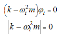
• ω_i - natural frequencies of the system;

• φ_i - natural modes of the system.

The system of equations is solved using the mode superposition method:

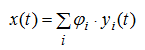
• y_i(t) - modal displacement coefficient.

We substitute Σφy_i(t) into the system equilibrium equation and multiply from the left by φ_i^T.

Using the orthogonality condition of the forms, we obtain:

• ξ_i - modal damping coefficient for the i - th mode;

• Г_i - modal participation coefficient for the i - th mode, which is determined by:

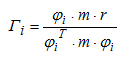
The equation differs from the equation of a single-mass oscillator only by the coefficient Г_i.

After the Fourier transform, this equation takes the form:

Transfer function for the i-th mode:

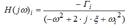
Transfer function modulus for the i-th mode:

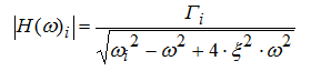
Power spectral density of the modal displacement coefficient i-th fashion:

• S_x″g(ω) - spectral density of the input action power.

Spectral density of the power of the i-th mode displacement:

Total spectral density of the power of displacement:

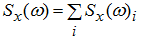
Root mean square deviation (1 sigma) of displacement:

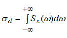
To find 2sigma, 3sigma, Nsigma, you need to multiply the 1sigma result by the corresponding N.