Search the documentation
Enter at least 2 characters
Enter at least 2 characters
 |
CAE Fidesys 9.0 Documentation |
Source - Boykov V.G., Gaganov I.V., Faizullin F.R., Yudakov A.A.. Simulation of the motion of the mechanical system consisting of the deformable elastic bodies by integrating two packages: Euler and Fidesys // Chebyshevsky collection, 2001. - v. 18, no. 3. - P. 131-153.
We consider the implementation of an interface for the calculations using finite element models in the form of elastic links to the PC EULER. This makes it possible to take into account the effect of elastic deformations of the links of the mechanism on the movement dynamics, as well as to quickly and conveniently consider the effect of changing the movement parameters and the mechanism structure on the stress-strain state in the detail.
division of nodes into interface (nodes of action of force elements and hinges and nodes, an approximate representation of the movement of which is undesirable) and internal;
calculation of static shapes from unit displacements along all degrees of freedom of interface nodes; >Calculation of natural vibration modes with clamped interface nodes;
building a modal matrix HF, reduced mass and stiffness matrices:
 , where MFEM,
CFEM - complete mass and stiffness matrices FEM-body models;
in this case, small elastic displacements of the body are approximated
by a set of admissible shapes: xn=HFω, where
xn – coordinates of all FEM-model nodes in the body's own
system of coordinates, ω – a set of modal dimension coordinates H,
where H – full number of forms used;
, where MFEM,
CFEM - complete mass and stiffness matrices FEM-body models;
in this case, small elastic displacements of the body are approximated
by a set of admissible shapes: xn=HFω, where
xn – coordinates of all FEM-model nodes in the body's own
system of coordinates, ω – a set of modal dimension coordinates H,
where H – full number of forms used;
 generalized eigenvalue problem for reduced matrices:
 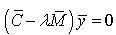 ; getting a
modal matrix HR, orthonormal with respect to complete matrices
model:
; getting a
modal matrix HR, orthonormal with respect to complete matrices
model: , then:
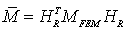 is single,
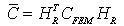 - is diagonal. Where in xn=HRω
.
- is diagonal. Where in xn=HRω
.The mentioned body's own coordinate system, in which elastic displacements are approximated by a set of admissible forms, is the so-called attached coordinate system (ACS) of the body. This is the coordinate system associated with the body. If the body does not perform elastic vibrations (relatively speaking, it is frozen), then the entire movement of the body is determined by the movement of the ACS. It is with respect to the ACS that the concept of small elastic displacements in the Craig-Bampton method is considered. For brevity, the basic inertial coordinate system will be called CS0.
Everywhere below, under the modal matrix H, generally speaking, we mean an arbitrary matrix of admissible forms, and the vector of modal coordinates ω is chosen in such a way that
xn=Hω (1)
Thus, a general independence of the used reduction method is achieved. In particular, it can be matrix HF or HR from Craig-Bampton model. It should be noted, however, that in order to ensure the correctness of further calculations, the linear relationship between the admissible and solid body shapes must be excluded in some way. This can be achieved, for example,when orthonormalizing the modal subspace in the Craig-Bampton method, one does not include the vibration modes with zero frequency in the modal matrix HR. The equations of dynamics of elastic bodies are derived from the Lagrange equation of the second kind:

where T – kinetic energy, U – potential, q– vector of generalized body coordinates, s – generalized force vector. For q we choose a set of two vectors: a six-dimensional vector (r,φ) ,characterizing the position of the ACS relative to CS 0, and the vector of modal coordinates ω. For any vectors a, b, ... we denote by (a, b, ...) their combining into a common vector. For the convenience of writing formulas and their analysis, we take as r and φ such vectors that:

where  – linear
and angular velocity of the ACS relative to CS0. Let
– linear
and angular velocity of the ACS relative to CS0. Let  -
be linear and angular acceleration of the ACS relative to CS0,
-
be linear and angular acceleration of the ACS relative to CS0,  .
.
Let N - be the number of all nodes of the FEM-model of the body, then
the number of degrees of freedom of the model is 6N, the size of the modal
matrix H is 6N × H, where H - is the number of shapes used. Index r corresponds
to translational displacements, φ to rotational, –
elastic; indices k and l - are node indices,
–
elastic; indices k and l - are node indices,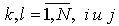 –
shape indices,
–
shape indices,  .
.
Let xn,k denote the six-dimensional vector of the k-node position in the UCS, Hk – the part of the modal matrix related to this node:

Let hk,i - denote the i-matrix column ;
;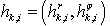 . Let us denote by
pk the initial position vector of the k-th node center relative
to the UCS. Then, taking into account (1), the position of the center
of the k-th node relative to CK0 at any moment of time can be written
in the form of:
. Let us denote by
pk the initial position vector of the k-th node center relative
to the UCS. Then, taking into account (1), the position of the center
of the k-th node relative to CK0 at any moment of time can be written
in the form of:

The point of derivating the elastic structures equations is to write formulas for calculating all the terms of the Lagrange equation (2). From the theory of the classical finite element method, an equation is known for calculating the kinetic energy of the FEM-model of a body:

where  – velocities
of all nodes of the body FEM-model, MFEM – complete mass matrix.
In the classical FEM, it is assumed that the body is not subject to large
motion as a whole, therefore both the velocities and the mass matrix are
written relative to the basic inertial CS. The main idea of using this
formula in the formulation considered in this article is as follows: the
complete mass matrix is constant in the body's own SC, that is, in the
ACS. This statement is obvious from the definition of the attached coordinate
system, since the motion of the ACS determines the movement of the body
as a whole, and all elastic displacements of the points of the body are
considered relative to the ACS.
– velocities
of all nodes of the body FEM-model, MFEM – complete mass matrix.
In the classical FEM, it is assumed that the body is not subject to large
motion as a whole, therefore both the velocities and the mass matrix are
written relative to the basic inertial CS. The main idea of using this
formula in the formulation considered in this article is as follows: the
complete mass matrix is constant in the body's own SC, that is, in the
ACS. This statement is obvious from the definition of the attached coordinate
system, since the motion of the ACS determines the movement of the body
as a whole, and all elastic displacements of the points of the body are
considered relative to the ACS.
All physical quantities within the framework of one formula, of course,
should be expressed in one coordinate system. In formula (4), it is convenient
to express the velocity vector in the ACS, since the
mass matrix is constant in the ACS. In this case, of course, the speeds
are recorded relative to the base CS0. Vector  ,
where
,
where  - is linear
and angular velocity of the k-th node relative to CS0. Taking into account
formula (2), it can be shown that:
- is linear
and angular velocity of the k-th node relative to CS0. Taking into account
formula (2), it can be shown that:

The “~” sign over a three-dimensional vector denotes the operation of
taking a skew-symmetric matrix for this vector; the “~” sign above the
opening parenthesis is applied to the result of the parenthesized expression.
If we introduce the matrices
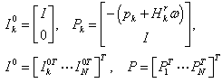 ,
,
then the velocity vector can be expressed as:

Let the complete mass matrix have an arbitrary form:
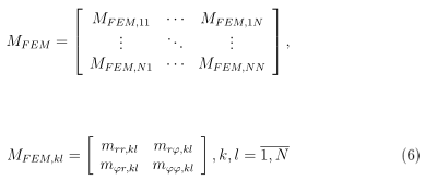
where mrr,kl, mrφ,kl, mφr,kl, mφφ,kl - are size 3 × 3 blocks. Substituting formulas (5) and (6) into formula (3), the expression for calculating the kinetic energy can be written in the form of:

Here M - is the generalized mass matrix. To write out formulas for calculating all of its components, you need to enter 18 matrices,presented in Table 1. Each sum here is the sum by the indices k, l, from 1 to N, that is,double sum over all body nodes. All these matrices are constant in the ACS.
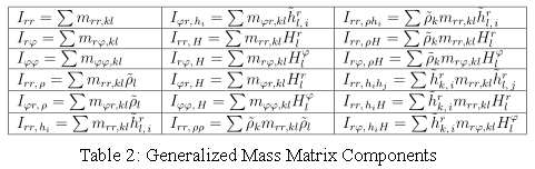 ,
,
Formulas for calculating blocks of the mass matrix can be written as:
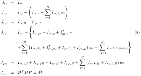
It is evident that Jrr, Jrω, Jωω - are constant in ACS, Jrφ, Jφω - linearly depend on ω, аnd Jφφ – quadratically. The mass matrix M in the ACS has a simple form:

Obviously, M is symmetric. From a comparison of formulas (3) and (7)
for calculating the kinetic energy, it is easy to obtain that if M FEM
is positively defined, then M is also positively defined.
So, the final formulas for calculating the generalized mass matrix have
been obtained. Substituting formulas (7) and (9) into the Lagrange equation
(2), one can show that: 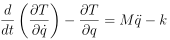
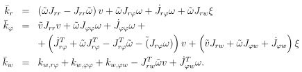
where k - is the vector of generalized inertial forces, which can be written in the ASC as:

If we introduce vectors kω,rφ, kω,φφ, kω,φω, whose components are equal:
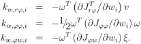
then the formulas for calculating the components of the vector of generalized inertia forces will be written as:
Consider further the remaining terms of the Lagrange equation (2). The total potential energy of the body is U=UC+Ug, where UC - is the potential energy of elastic deformations, Ug – is the potential energy of gravity. Using the formula for calculating the elastic deformation energy of the FEM body model:
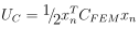
and taking into account that the full stiffness matrix is constant in
the ACS (similar to the mass matrix), it can be shown that: 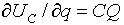 , where
 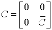 - is generalized
stiffness matrix,
- is generalized
stiffness matrix, 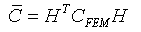 -
is reduced stiffness matrix. This means that the generalized elastic force
is:
-
is reduced stiffness matrix. This means that the generalized elastic force
is:

If we denote by gr gravitational acceleration vector,
it can be shown that ,
where g=(gr;0;0). Therefore, the generalized force of gravity
is:
,
where g=(gr;0;0). Therefore, the generalized force of gravity
is:

The mathematical model of damping is constructed by known methods based
on the Rayleigh dissipative function: ,where D is generalized
damping matrix:
,where D is generalized
damping matrix: . Reduced
damping matrix
. Reduced
damping matrix  is
obtained either by the Rayleigh method:
is
obtained either by the Rayleigh method: 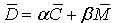 ,
where α and β – some constants, or based on the representation of free
vibrations of the body by a set of independent equations of motion with
one degree of freedom, then
,
where α and β – some constants, or based on the representation of free
vibrations of the body by a set of independent equations of motion with
one degree of freedom, then ,
where
,
where  – critical damping
factor of the corresponding shape, ωk– its natural vibration
frequency. In this case, the generalized damping force is:
– critical damping
factor of the corresponding shape, ωk– its natural vibration
frequency. In this case, the generalized damping force is:

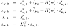
Let force f k and moment m k be applied to the
k-interface node at a point spaced from this node by the vector ρ f,
k then - is
applied force reduced to the center of the node. From the condition of
equality of virtual jobs on possible displacements along generalized coordinates,
we obtain (the summation is carried out over all the nodes of the body,
to which the forces are applied):
- is
applied force reduced to the center of the node. From the condition of
equality of virtual jobs on possible displacements along generalized coordinates,
we obtain (the summation is carried out over all the nodes of the body,
to which the forces are applied):
Bidirectional ties applied to an elastic body are modeled similarly to ties to solid bodies. The principles of constructing constraint equations are discussed in detail in the article [2]; we will briefly list them here. General view of the constraint equation:
 ,
,
where  – acceleration,
speed and position of the i-th local coordinate system (LCS) of the connection
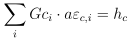
relative to SK0. Having differentiated, one can obtain an equation for
calculating the accelerations in connection (the summation is carried
out for all LCS of the given connection):
– acceleration,
speed and position of the i-th local coordinate system (LCS) of the connection
relative to SK0. Having differentiated, one can obtain an equation for
calculating the accelerations in connection (the summation is carried
out for all LCS of the given connection):
 ,
,
where 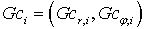 – the matrix
of the derivatives of the link residuals by the motions of the i-th link
LCS, hc– link acceleration residual vector, determined depending
on the link type. By expressing the parameters of the LCS, which is associated
with a solid or an elastic body, through the parameters of this body,
we obtain:
– the matrix
of the derivatives of the link residuals by the motions of the i-th link
LCS, hc– link acceleration residual vector, determined depending
on the link type. By expressing the parameters of the LCS, which is associated
with a solid or an elastic body, through the parameters of this body,
we obtain:
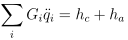 ,
,
where  – the matrix
of residual derivatives of the i-bond LCS with respect to the generalized
coordinates of the corresponding body (generalized Jacobian of the bond).
If the i-th LCS of the connection belongs to the k-interface node of the
body and is spaced from it to the vector ρ c , then omitting
the index i, we can write:
– the matrix
of residual derivatives of the i-bond LCS with respect to the generalized
coordinates of the corresponding body (generalized Jacobian of the bond).
If the i-th LCS of the connection belongs to the k-interface node of the
body and is spaced from it to the vector ρ c , then omitting
the index i, we can write:
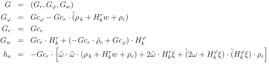
The generalized forces of the bonds reaction can be expressed by the formula (see [2]):
 ,
,
where λ – power factors in connections.
Thus, all terms of the Lagrange equation (2) have been considered. Combining them together, we obtain an equation for calculating the motion of the deformed body in general setting:

where M,C,D - are generalized matrices of mass, stiffness and damping, k is a vector of inertia forces,Sg– generalized gravity, Sa – generalized active forces, R – bond reaction forces. Equation (11) can be written as:
 ,
,
where – sum of generalized
forces of elasticity, damping, gravity and active concentrated forces.
– sum of generalized
forces of elasticity, damping, gravity and active concentrated forces.
It has the same form as the generalized equation of motion of a rigid body.
This makes it possible to simulate dynamics of an elastic structure as
part of a multicomponent mechanical system.