Search the documentation
Enter at least 2 characters
Enter at least 2 characters
 |
CAE Fidesys 9.0 Documentation |
Source - Boykov V.G., Gaganov I.V., Faizullin F.R., Yudakov A.A.
Motion Simulation of a Mecanical System
Consisting of Deformable Elastic Bodies by Integration
of Two Packages: EULER AND FIDESYS// Chebyshevsky collection, 2001. - v.
18, no. 3. - P. 131-153.
The KAMAZ-5308 vehicle model consists of a Carrier module assembly,
which includes the Frame_Elastic unit, and other units: Cargo,
Cab, Power transmission unit, Hitch, Support-running module, Steering.
Part of the model geometry was created in the NX program.
An image of a model with an elastic frame is shown in Fig. 1.
The design diagrams of the front and rear suspension are shown in Fig.
2 and Fig. 3.
The following assumptions are made in the suspension models:
1.the axle and axle arms are considered absolutely rigid;
2. There are no deformations and friction in the suspension joints.
The KAMAZ-5308 vehicle uses a steering system that turns the wheels of
one axle using
a continuous trapezoid and a steering mechanism with a rotary movement
of the output link.
The model diagram is shown in Fig. 4.
The finite element model of the KAMAZ-5308 carrier module consists of the following elements:
1. Product frame
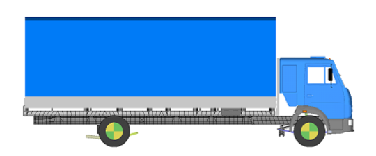
Fig. 1: View of the KAMAZ-5308 car model with included FE frame model
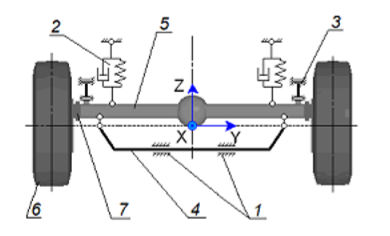
Fig. 2: Diagram of front suspension model: 1 – basic link; 2 – elastic damping element; 3 - trailing arm; 4 – stabilizer; 5 – bridge; 6 - wheel; 7 - pin
2. Product platform
In the simulation, the following assumptions were made:
Fillet radii are not taken into account;
Suspension brackets, cabins are considered very stiff compared to the structure itself;
Technological holes are not taken into account.
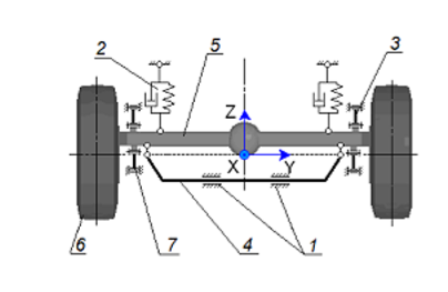
Fig. 3: Scheme of the rear suspension model: 1 – basic link; 2 – elastic damping element; 3 - trailing arm; 4 - stabilizer; 5 – bridge; 6 - wheel; 7 - additional trailing arm
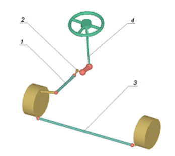
Fig. 4: Steering model diagram: 1 - longitudinal thrust; 2 - bipod; 3 - transverse thrust; 4 - steering column
The model uses the SI measurement system. The model consists of 5415
four-node cladding elements of type CQUAD4. Material (steel)
is given by Young's modulus, Poisson's ratio and density.
26 nodes are specified as interface for dynamic reduction.
They correspond to the places of attachment to the frame of the rest of
the vehicle structure - suspension, cargo and cab.
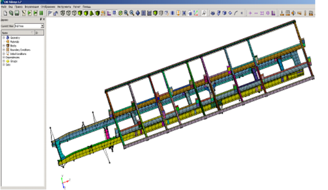
Fig. 5: General view of the model opened in Fidesys
The process begins by uploading the model to Fidesys. Fidesys supports
many formats, as well as the ability to create the model itself in Fidesys.
If you have a ready-made model, after loading it, you just need
to select the interface nodes. In the next implementation of the bundle,
if there is a ready-made model, it is not necessary to launch the Fidesys
interface. It is planned that the user will be able to run the calculation
from the Euler interface.
Thus, when studying this technology, the user does not need to understand
the interfaces of both programs at the same time.
The algorithm will automatically pull the model and all the necessary calculations
into Fidesys.
It is necessary to determine the number of degrees of freedom for the interface
nodes. In our example, the model completely
consists of two-dimensional parts and, accordingly, the total degrees of
freedom will be 26 · 6 = 156.
Following the Craig-Bampton algorithm, it is necessary to make 156 calculations
for statics, where each calculation represents the following - all interface
nodes are fully secured except for one; this node produces a single displacement
by one of the degrees of freedom,
but according to the remaining degrees of freedom, the knot will also be
completely fixed.
One separate calculation for natural frequencies on the model, where all
interface knots are fixed.
Separately, the model geometry, mass and stiffness matrices are unloaded.
In the presence of rigid links, the matrices are reduced by rows corresponding
to the dependent degrees of freedom.
For transmission of sparse matrices,we chose the .HB format.
For the transfer of own and static forms, a special .cbm format was developed.
As a result, we get 4 files: M_CCS.hb and K_CCS.hb - mass and stiffness
matrices, respectively.
geometry.vtk - file with model geometry.
forms.cbm - file with own and static forms.
If there are hard links, information about them is placed in the vtk file.
In the case of our example, all files in total occupy about 102 megabytes.
All of these files are read by EULER.
In calculating the dynamics, the first 10 eigenforms of an elastic body
are used.
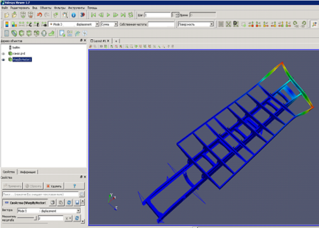
Fig. 6: Proprietary shapes used in dynamics analysis
The model is designed to determine the maximum speed of maneuver when
changing lanes on a limited section of the road,
at which there is no separation of the wheels from the road or the exit
of the vehicle outside the overall corridor. This type of test is regulated
by GOST Р 52302-2004.
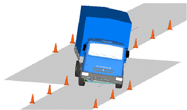
Fig. 7: Model appearance
During the calculation, the machine is controlled by a feedback control
system.
To simulate the test, we use the marked corridor shown in Fig. 8.
Polygon cohesion parameters are set by the user.
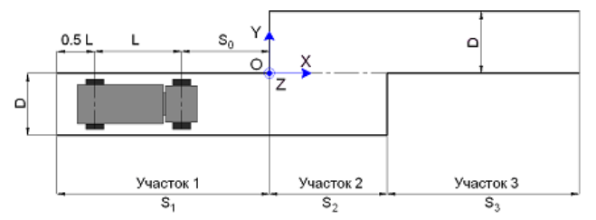
Fig. 8: Layout of the "Rearrangement" test model section
The CM is told the initial speed V x0 of movement on section
1 of the marked corridor.
This speed, if desired by the user, can be maintained throughout the test
using the speed regulator.
In section 1 of the marked corridor, the steering wheel is held in neutral
position.
From the moment the point in the middle of the first CM axis crosses the
boundary between sections 1 and 2, the operation of the control algorithm,
described above, begins.
In section 3, the steering wheel is held in neutral.
In all sections, the exit of the CM outside the marked corridor is monitored
by the position of special dimension points fixed on the CM frame along
both sides. Dimensional points are located in the region of each axis
of the CM at the height of the wheel centers and at a distance of half
of the specified overall width of the CM from its longitudinal plane.
Wheel separation from the road is monitored using tire deflection sensors.
The end of the race is done automatically after passing the KM
distance:
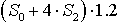 .
.
If the initial speed V x0 KM is less or equals 0.1 m / s, the race ends after 10 s of model time.
To test the operation of elastic links and the effect of taking into
account the elasticity of links on the calculation results for the KAMAZ-5308
vehicle,
calculations of the "Rearrangement" tests were carried out for
cases with a rigid and an elastic frame. The test was carried out at a
vehicle speed of 30 km / h. and 55 km / h
The length of the conversion section is 20 m. Fig.4 - Fig. 11 show the
results of the "Rearrangement" test at a speed of 30 km / h
(black lines - elastic frame, red lines - rigid frame). Also, the values
of elastic displacements were obtained for the frame (not taking into
account the displacements of the frame as a whole). The front part of
the frame experiences the greatest elastic displacements, the maximum
value is 11mm.
Fig. 4 - Fig. 11 show the results of the "Rearrangement" test
at a speed of 55 km / h (black lines - elastic frame, red lines - rigid
frame). For the frame, the values of elastic displacements were obtained
(not taking into account the displacements of the frame as a whole). The
front part of the frame experiences the greatest elastic displacements,
the maximum value is 21 mm. In this article, the use of the FEM model
was used to take into account the influence of the dynamics of the vehicle
movement as a whole on the stress-strain state of the frame.
Thus, the FEM-model prepared in CAE Fidesys can be inserted into the EULER
software and calculated as part of a multicomponent
mechanical system within the framework of the classical finite element
method and using the Craig-Bampton reduction method.
For demonstration, the dynamics of the model was calculated using the example
of the `` Rearrangement '' test for a KAMAZ-5308 vehicle with an elastic
frame.
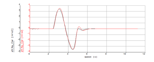
Fig. 9: Lateral acceleration for a rigid and resilient frame at test speed 30 km / h
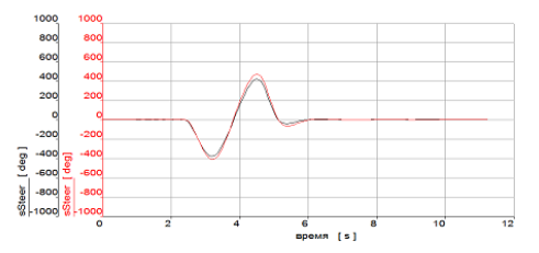
Fig. 10: Steering angle for a rigid and resilient frame at test speed 30 km / h
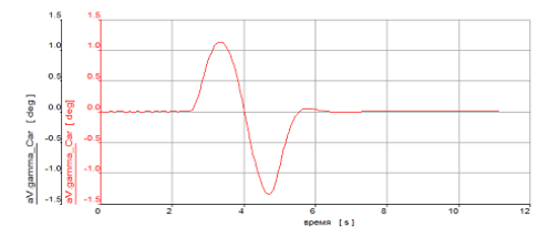
Fig. 11: Angle of lateral roll for a rigid and resilient frame at test speed 30 km / h
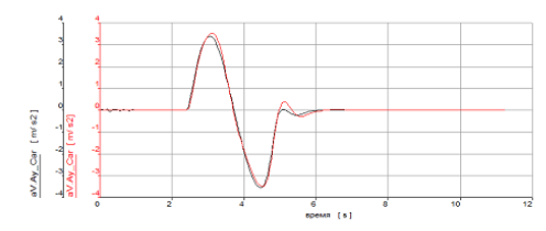
Fig. 12: Lateral acceleration for tight and elastic frame at a test speed of 55 km / h
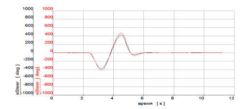
Fig. 13: Steering angle for firm and an elastic frame at a test speed of 55 km / h
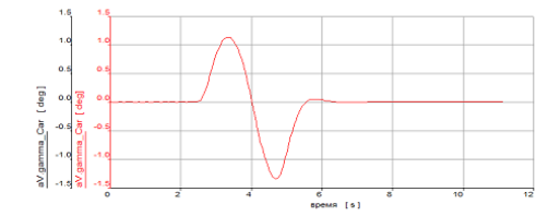
Fig. 14: Roll angle for rigid and an elastic frame at a test speed of 55 km / h