Effective Property Calculation and its Results

CAE Fidesys supports the calculation of such effective properties as:

Effective Elasticity Moduli;

(taking into account the preliminary loading of the model and with the possibility of setting a tabular / functional dependence of material properties on any parameters);
Effective Density and Porosity;
Effective Coefficients of Thermal Expansionon;
Effective Biot Coefficients;
Effective Thermal Conductivity;
Effective Permeability Coefficients.

For any type of calculation, you can set the contact interaction between the constituent parts of the representative volume or the periodicity cell

1. Effective Elasticity Moduli

To set effective linear elastic properties calculation tick "Elasticity" in the settings for calculating effective properties. To calculate effective properties the model undergoes a series of strains. The following types of strains are used:

tension (along each of the coordinate axes);
shears (in each of the coordinate planes).

The deformation value is 0.2% for all types. Thus, in the three-dimensional case, the representative volume (periodicity cell) is solved 6 static boundary value problems of elasticity theory, 3 problems in two–dimensional. All problems are solved in a geometrically linear formulation.

Consideration of preload in the calculation of effective linear elastic The characteristics are indicated by a check mark "Preloaded model". The preload may be, for example, the pore pressure for porous material, heating, causing temperature stresses, etc. The boundary conditions determining the preloading of the model are given by by the user in the interface. At the same time, they should not be applied to the outer boundary of a representative volume (periodicity cells) – surfaces/lines obtained as a result of "cutting" a fragment from the material in the form of a rectangular parallelepiped (rectangle) and parallel coordinate planes/axes.

To account for the preload on the model, an additional static problem of elasticity theory – a total of 7 problems in three dimensions are obtained. There are 4 tasks in the two-dimensional case. All tasks are solved in this case. taking into account geometric nonlinearity.

Effective properties are evaluated in the form of the generalized Hook's law:

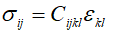
The result of the calculation is effective elastic modules C_ijkl displayed to the command line and in the file called Cijkl.txt in the working directory. The modules are evaluated in the coordinate system where the calculation was carried out (in which coordinate planes are parallel to the edges of calculation model).

Modules C_ijkl contain 21 independent constants – it is often more than it is necessary to describe effective properties of the tested heterogeneous material. That is why there is a possibility of the automatic conversion of the obtained effective elastic modules into constants of orthotropic, transversally isotropic or isotropic material. After completing the calculation of the effective properties, the window «Process effective properties data» opens. In the window, obtained effective elastic modules C_ijkl are shown at the bottom right in the form of a symmetric matrix sized 6x6 (the matrix part below the main diagonal is not displayed because of the symmetry).

If the calculated effective elastic moduli are unphysical, immediately after opening the data processing window a message will pop up, warning that the matrix is not symmetric with sufficient accuracy or is not positive definite. In this case you should check again the correct choice of model for calculation:

if it is a rectangular parallelepiped with faces parallel to the coordinate planes;
in the two-dimensional case, if it is a rectangle with sides parallel to the coordinate axes;
if it is a periodicity cell in case of calculation with periodic boundary conditions.

If the model is correct, it is necessary to improve (grind) the grid.

When the calculation is complete, the window opens automatically. If the user closes it, it can be re-opened in the mode Material -> Effective Properties:

The user can assess whether the matrix with obtained C_ijkl corresponds to orthotropic materials with the acceptable tolerance. For the exact orthotropic material, the matrix should look as follows (where the letters X denote those components that can be nonzero).

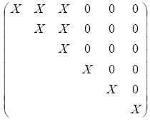
But, since the components of the matrix are the result of a numerical calculating effective properties – they usually contain some error. If, from the user's point of view, the matrix corresponds to an orthotropic material with acceptable accuracy, you can select the type of elastic properties "Orthotropic" and click the "Process data" button, as a result of which the values will be calculated nine constants of orthotropic material. If the material is not orthotropic with sufficient accuracy, or if the orthotropic constants turned out to be non-physical – when you click the "Process data" button, a window opens with a corresponding warning.

If the orthotropic constants do not depend on the direction (i.e., for example, different Young's modules are the same or differ from each other within an acceptable margin of error), then you can select the "Isotropic" type of material and click the "Process data" button again. Two constants of the isotropic material will be calculated – the Young's modulus and the Poisson's ratio. If the material is not isotropic with sufficient accuracy, or if the Young's modulus and/or the Poisson's ratio turned out to be unphysical – when you click the "Process" button data" opens a window with a corresponding warning.

It is possible to calculate the effective elastic characteristics of an inhomogeneous material, the elastic properties of the components of which have a tabular/functional relationship. depends on any variables. For example, you can set a property dependency depending on the temperature, set uniform heating of the representative volume (periodicity cells) – and calculate effective elastic properties at this temperature. Moreover, if at least one of the materials has a non–zero coefficient of thermal expansion, the effective properties will be considered without taking into account the set temperature.

2. Effective Density and Porosity

Density is an additive quantity. Therefore, the effective density is calculated as the mass of the model divided by the effective volume (including pores and voids in the material). Density is calculated automatically for any calculation of effective characteristics.

Similarly for porosity. Effective porosity is calculated as the ratio of pore volume to effective volume (including pores and voids in the material).

3. Effective Coefficients of Thermal Expansion

Calculation of effective coefficients of linear thermal expansion is set in the settings for calculating effective properties by checking the box "Thermal expansion". To calculate the effective coefficients of thermal expansion, the model is subjected to uniform heating. The heating value is 1 K.

Effective thermal expansion is estimated as:

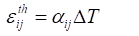
The results of the calculation are effective coefficients of thermal expansion,which are output to the command line and to a JSON file called EffProps.json located in the working directory. Coefficients are calculated in that coordinate system, in which the calculation was carried out (to the coordinate planes / axes of which the faces / sides of the calculation model are parallel).

Coefficient matrix α_ij contains 6 independent constants, often this is more than enough to describe the effective linear thermal expansion of the studied heterogeneous material. Therefore, it is possible to automatically recalculate obtained effective coefficients of linear thermal expansion into constants of an orthotropic or isotropic material. The window "Process data on effective properties" will appear after the calculation is completed. You may see the effective coefficients of thermal expansion α_ij on the “Temperature” tab on the right in the form of a symmetric matrix of thermal expansion of size 3x3 (the part of the matrix below the main diagonal is not displayed due to symmetry).

If the calculated effective thermal conductivities are unphysical, immediately after opening the data processing window, the system will show a warning that the matrix α_ij is not symmetric with sufficient accuracy or is not positively definite. In this case you should check again the correct choice of model for calculation:

if it is a rectangular parallelepiped with faces parallel to the coordinate planes;
in the two-dimensional case, if it is a rectangle with sides parallel to the coordinate axes;
if it is a periodicity cell in case of calculation with periodic boundary conditions.

If the model is correct, it is necessary to improve (grind) the grid.

The user can assess whether the matrix with obtained α_ij corresponds to orthotropic materials with the acceptable tolerance. For the exact orthotropic material, the matrix should look as follows (where the letters X denote those components that can be nonzero).

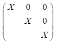
Since the components of the matrix are the result of numerical calculation of effective properties - they tend to contain some errors. If, from the user's point of view, the matrix corresponds to orthotropic materials with acceptable tolerance, select the «Orthotropic» type of material and click «Process Data», and the system will calculate nine constants of orthotropic material. If the material is not orthotropic with sufficient accuracy or if orthotropic constants turned out to be unphysical, when you click "Process data” the system will show you a message with a warning.

If orthotropic constants do not depend on the direction (i.e., for example, different Young's moduli are the same or differ from each other within the acceptable error) then you can select the type of material «isotropic» and click «Process data» again. The system will calculate two constants of an isotropic material – Young’s Modulus and Poisson's Ratio. If the material is not isotropic with sufficient accuracy or if Young's modulus and / or Poisson's ratio are unphysical, when you click "Process data” the system will show you a message with a warning.

4. Effective Biot Coefficients

The calculation of the effective Biot coefficients is set in the settings for calculating the effective properties by checking the Poroelasticity checkbox. To calculate the effective Biot coefficients, fixing boundary conditions are imposed on the outer boundary of the model (i.e., not allowing its deformation). All internal surfaces are subjected to the same pressure.

The effective poroelasticity of a material is estimated in the form of the Biot-Terzaghi law:

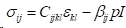
The result of the calculation is the effective Biot coefficients output to a JSON file named EffProps.json located in the working directory. The coefficients are calculated in the coordinate system in which the calculation was performed (the coordinate planes/axes of which are parallel to the faces/sides of the calculation model).

The matrix of coefficients contains 6 independent constants, which is often more than enough to describe the effective poroelasticity of the investigated inhomogeneous material containing pores. Therefore, it is possible to automatically recalculate the obtained effective Biot coefficients into the constants of an orthotropic or isotropic material. When the calculation is completed, the "Process Effective Properties Data" window also appears. The effective Biot coefficients are shown on the Poroelasticity tab on the right as a symmetrical 3x3 poroelasticity matrix (the portion of the matrix below the main diagonal is not displayed due to symmetry).

If the calculated effective combat coefficients are not physical, immediately after opening the data processing window, a window appears with a corresponding warning about the matrix asymmetry with sufficient accuracy. In this case, one should once again check the correctness of the choice of the model for calculation: whether it is a rectangular parallelepiped with faces parallel to the coordinate planes (in the two-dimensional case, a rectangle with sides parallel to the coordinate axes) , and whether it is a periodicity cell in the case of calculation with periodic boundary conditions. If the model is built correctly, it is likely that the mesh needs to be improved (refine).

The user can evaluate whether the matrix corresponds to the received orthotropic material with the accuracy that satisfies him. For an exact orthotropic material, this matrix should look like this (here X denotes those components that can be non-zero).

But, since the matrix components are the result of a numerical calculation of the effective properties, they usually contain some error. If, from the user's point of view, the matrix corresponds to an orthotropic material with acceptable accuracy, you can select the poroelastic property type "Orthotropic" and click the "Process Data" button, which will calculate the three orthotropic material constants. If the material is not orthotropic with sufficient accuracy, or if the Biot orthotropic coefficients are found to be non-physical, pressing the "Process data" button will open a window with a corresponding warning.

If the orthotropic constants do not depend on the direction (different Biot coefficients are the same or differ from each other within the acceptable error), then you can select the material type "Isotropic" and click the "Process data" button again. One constant will be calculated - the isotropic coefficient of the Biomaterial. If the material is not isotropic with sufficient accuracy, pressing the "Process data" button will open a window with a corresponding warning.

5. Effective Thermal Conductivity

To set the calculation of the effective thermal conductivity tick “Thermal conductivity”in the settings for calculating the effective properties. To calculate the effective thermal conductivity coefficients, the model undergoes a series of heatings: the system sets different temperatures corresponding to a certain temperature gradient in the model on its faces. The system uses gradients directed along each coordinate axis. The effective thermal conductivity of the material is estimated in the form of the Fourier law of thermal conductivity:

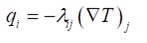
The result of the calculation is the effective thermal conductivity coefficients λ_ij, output to the command line and to a JSON file with the name EffProps.json located in the working directory. The program calculates the coefficients in the coordinate system in which the calculation was carried out (to the coordinate planes / axes of which the faces / sides of the calculation model are parallel).

The coefficient matrix λ_ij contains 6 independent constants. Often this is more than enough to describe the effective linear thermal conductivity of the studied inhomogeneous material. Therefore, it is possible to automatically convert the obtained effective coefficients of linear thermal conductivity to the constants of an orthotropic or isotropic material. After the calculation is completed, the “Process data by effective properties” window also appears. Temperature tab, bottom right, shows effective thermal conductivity λ_ij coefficients in the form of a symmetric thermal conductivity matrix of size 3x3 (a part of the matrix below the main diagonal is not displayed due to symmetry).

If the calculated effective thermal conductivities are unphysical, immediately after opening the data processing window, the system will show a warning that the matrix λ_ij is not symmetric with sufficient accuracy or is not positively definite. In this case you should check again the correct choice of model for calculation:

if it is a rectangular parallelepiped with faces parallel to the coordinate planes;
in the two-dimensional case, if it is a rectangle with sides parallel to the coordinate axes;
if it is a periodicity cell in case of calculation with periodic boundary conditions.

If the model is correct, it is necessary to improve (grind) the grid.

The user can assess whether the matrix with obtained corresponds to orthotropic materials with the acceptable tolerance. For the exact orthotropic material, the matrix should look as follows (where the letters X denote those components that can be nonzero).

If orthotropic constants do not depend on the direction (different coefficients of thermal conductivity are the same or differ from each other within the acceptable error) then you can select the type of material "Isotropic" and click "Process Data" again. The system will calculate one constant - isotropic coefficient of linear thermal conductivity of the material. If the material is not isotropic with sufficient accuracy, when you click "Process data” the system will show you a message with a warning.

The calculation of the effective thermal conductivity of an inhomogeneous material can be carried out separately or together with calculations of effective elastic properties (in the second case, in the calculation settings it is necessary to tick the checkboxes “Elasticity” and “Thermal conductivity”). If the thermal expansion coefficients of at least one material in the model are specified in the joint calculation, the effective moduli of elasticity, the effective coefficients of thermal expansion, and the effective coefficients of thermal conductivity will be calculated. In the window for processing results, both thermal conductivity coefficients and thermal expansion coefficients are located on the “Temperature” tab.

Effective thermal conductivity coefficients are calculated only for the case of linear thermal conductivity. The calculation is impossible if the temperature dependence of the thermal conductivity coefficients is specified for at least one of the components of the investigated inhomogeneous material. The calculation of the effective thermal conductivity of an inhomogeneous material can be carried out separately or together with the calculation of the effective elastic properties and / or effective coefficients of thermal expansion (in the calculation settings, you can select any of the checkboxes "Elasticity", "Thermal expansion" and "Thermal conductivity"). In the results processing window, both the thermal conductivity and thermal expansion coefficients are located on the "Temperature" tab.

6. Effective Permeability Coefficients

The calculation of effective permeability is set in the settings for calculating effective properties by checking the "Permeability" box. In order to calculate the effective permeability coefficients, different pore pressures corresponding to different pore pressure gradients in the model are set on the faces of the model. Gradients directed along each coordinate axis are used.

The effective permeability of the material is estimated in the form of Darcy's law:

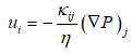
The calculation results in effective permeability coefficients k_ij that are output to the command line and to a JSON file named EffProps.json located in the working directory. The coefficients are calculated in the coordinate system in which the calculation was performed (the coordinate planes/axes of which are parallel to the faces / sides of the calculated model).

The coefficient matrix k_ij contains 6 independent constants – often this is more than enough to describe the effective linear permeability of the inhomogeneous material under study. Therefore, it is possible to automatically convert the obtained effective linear permeability coefficients into constants of an orthotropic or isotropic material. After the calculation is completed, the "Process data by effective properties" window appears. The effective permeability coefficients k_ij are shown on the Poroelasticity tab at the bottom right in the form of a 3x3 symmetric permeability matrix (the part of the matrix below the main diagonal is not displayed due to symmetry).

If the calculated effective permeability coefficients are non–physical, immediately after opening the data processing window, a window appears with a corresponding warning that the matrix k_ij is not symmetric with sufficient accuracy or is not positively defined. In this case, it is necessary to check again the correctness of the choice of the model for calculation: whether it is a rectangular parallelepiped with faces parallel to coordinate planes (in the two–dimensional case, a rectangle with sides parallel to coordinate axes), and whether it is a periodicity cell in the case of calculation with periodic boundary conditions. If the model is built correctly, it is probably necessary to improve (grind) the grid.

The user can evaluate whether the matrix with the obtained k_ij orthotropic material corresponds with satisfactory accuracy. For an accurate orthotropic material, this matrix should look like this (here the letters X indicate those components that may be non-zero).

But, since the components of the matrix are the result of numerical calculation of effective properties, they usually contain some error. If, from the user's point of view, the matrix corresponds to the orthotropic material with acceptable accuracy, you can select the type of temperature properties "Orthotropic" and click the "Process data" button, as a result of which three constants of the orthotropic material will be calculated. If the material is not orthotropic with sufficient accuracy, or if the orthotropic linear permeability coefficients have turned out to be non–physical, clicking the "Process data" button opens a window with an appropriate warning.

If the orthotropic constants do not depend on the direction (different permeability coefficients are the same or differ from each other within an acceptable margin of error), then you can select the type of material "Isotropic" and click the "Process data" button again. One constant will be calculated – the isotropic coefficient of linear permeability of the material. If the material is not isotropic with sufficient accuracy, clicking the "Process data" button will open a window with a corresponding warning.

>>>>> Processing results and exporting effective material