CAE Fidesys 9.0 Documentation

Analysis of a Beam Subject to Random Vibration Specified by Power Spectral Density

Dynamic response of a system consisting of two massless mutually perpendicular beams and point masses under the influence of random vibration. For a given damping level ζ = 3% determine the dynamic response of the structure when exposed to random vibration in the form of white noise, specified as base acceleration power spectral density.

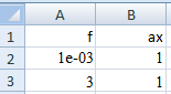
To carry out the analysis, you need to prepare a file in *.csv format. The file should contain a table where the first column contains frequency values ​​(Hz), subsequently – displacement (speed, acceleration). You must specify the column names:

• f - frequency;
• ax – acceleration along the Ox axis.

This table is created as a CSV file and then imported into FidesysViewer (the image shows an example of setting a table in Excel).

Note: Microsoft Excel can open a csv file like this:

those. without splitting the file into pillars and listing the values ​​of the lines of the file through comma.

To split text in rows into corresponding columns, you need to list separator settings of your operating system add a comma.

It is worth noting that if the settings are not changed, the file will not download correctly.  

Geometry creation

1. Create a straight line.

On the command bar, select the module for constructing geometry (Mode - Geometry, Entity - Curve, Action - Create).

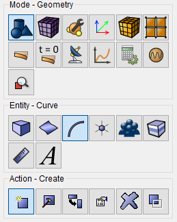
From the drop-down list, select Line.

In the Build Using panel, select Location and Direction.

Next, provide the necessary data to create the first line:

• Location: 0 0 0 (separated by space);

• Direction: 0 1 0;

• Length: 2.

Click Apply.

2. Provide the necessary information to create the second line:

• Location: 0 2 0 (separated by space);

• Direction: 1 0 0;

• Length: 2.

Click Apply.

3. Merge the vertices on the resulting lines.

On the command bar, select the module for constructing geometry (Mode - Geometry, Entity - Vertex, Action - Merge).

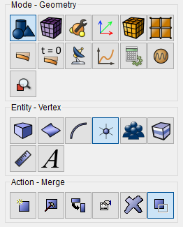
Set the following parameters:

• Vertex ID(s): 2 3.

Click Apply.

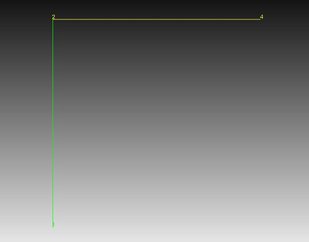
The result is a beam structure:

Meshing

1. On the command bar, select the mesh module (Mode — Mesh, Entity — Curve, Action — Mesh).

Set the following parameters:

• Select Curves: all;

• Select the mesh construction method: Equal;

• Interval;

• Interval: 10.

Click Apply Size.

Click Apply Mesh.

Setting the material and properties of blocks

1. Set the material.

In the command bar, select the module for specifying material properties (Mode - Material, Entity - Material Management).

In the opened widget Material management in the middle column specify the material name Mat1.

In the properties column, open the Elasticity list and drag the name Isotropic Material to the Material properties column.

In the properties column, open the General list and drag the name Density in the Material Properties column.

Fill in the properties as follows:

• Young's modulus: 2e+11;

• Poisson ratio: 0.33;

• Density: 1e-07.

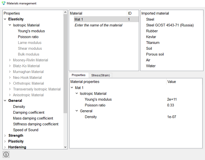
Click Apply.

Close the Materials management window.

2. Create the first block. Select the entity to be merged to block: Curves.

On the command bar, select the block management module (Mode - Blocks, Entity - Block, Action - Add).

Set the following parameters:

• Block ID: 1;

• Entity List: Curve;

• Entity ID(s): 1 2.

Click Apply.

3. Set block parameters.

On the command bar, select the block management module (Mode - Blocks, Entity - Block, Action - Block properties/parameters).

Set the following parameters:

• Block ID(s): 1;

• Category: Beam;

• Material: Mat1;

• Coordinate System: Global Cartesian;

• Order: 1.

Set the properties of the beam, to do this, click on the button .

Set the following parameters:

• Select profile: Custom Section;

• Y Eccentricity: 0;

• Z Eccentricity: 0;

• Inertia moment I_y: 4e-07;

• Inertia moment I_z: 4e-07;

• Inertia moment I_p: 0;

• Inertia moment I_yz: 0;

• Inertia moment on torsion It: 0;

• Area: 0.002242;

• Max Y coordinate: 0;

• Max  Z coordinate: 0;

• Shear coefficient YY: 1;

• Shear coefficient ZZ: 1;

• Shear coefficient ZY: 0;

• Shear center Y: 0;

• Shear center Z: 0;

• Warping constant I_ω: 0.

Click Apply. Close the Set Beam Properties window.

Click Apply.

4. Create a second block. Select the entity to be merged to block: Vertices.

On the command bar, select the block management module (Mode - Blocks, Entity - Block, Action - Add).

Set the following parameters:

• Block ID: 2;

• Entity List: Vertex;

• Entity ID(s): 2.

5. Set block parameters.

On the command bar, select the block management module (Mode - Blocks, Entity - Block, Action - Block properties/parameters).

Set the following parameters:

• Block ID(s): 2;

• Category: Lumped Mass;

• Coordinate System: Global Cartesian.

Set the properties of the point mass, to do this, click on the button .

Set the following parameters:

• Mass: 100;

• Inertia moment: 0.

Click Apply. Close the Set Lumped Mass window.

Click Apply.

6. Create a third block. Select the objects to be merged to block: Vertices.

On the command bar, select the block management module (Mode - Blocks, Entity - Block, Action - Add).

Set the following parameters:

• Block ID(s): 3;

• Entity List: Vertex;

• Entity ID(s): 4.

7. Set block parameters.

On the command bar, select the block management module (Mode - Blocks, Entity - Block, Action - Block properties/parameters).

Set the following parameters:

• Block ID(s): 2;

• Category: Lumped Mass;

• Coordinate System: Global Cartesian.

Set the properties of the point mass, to do this, click on the button .

Set the following parameters:

• Mass: 200;

• Inertia moment: 0.

Click Apply. Close the Set Lumped Mass window.

Click Apply.

Setting boundary conditions

1. Secure vertex A for all linear displacements and rotations.

On the command panel, select the boundary conditions module (Mode - Boundary Conditions, Entity - Displacement, Action - Create).

Set the following parameters:

• Entity List: Vertex;

• Entity ID(s): 1;

• Degrees Of Freedom: All.

Click Apply.

2. Fix the entire beam by linear displacement along the Z axis.

Set the following parameters:

• Entity List: Curve;

• Entity ID(s): all;

• Degrees Of Freedom: Z-Translation Disp.

Click Apply.

Starting calculation

1. Set general settings for modal analysis.

On the command bar, select the calculation settings module (Mode - Calculation Settings , Calculation Settings - Spectrum Analysis, Spectrum analysis - General).

Set the following parameters:

• Dimensions: 3D;

• Type: Random Vibration;

• Number of Eigenmodes: 2.

Click Apply.

Click Start Calculation.

2. In a pop-up window select a folder to save the result and enter the file name.

3. In the case of a successful calculation, the console displays the message: Calculation finished successfully at "date" "time".

Results analysis

1. Open the file with the results. There are three ways to do that.

• Click Ctrl+E.

• From the main menu, select Calculation. Click Open Results.

• Select Results on Command Panel (Mode - Results). Click Open results.

The Fidesys Viewer window will appear in which you can view with the calculation results.

Starting on random vibration

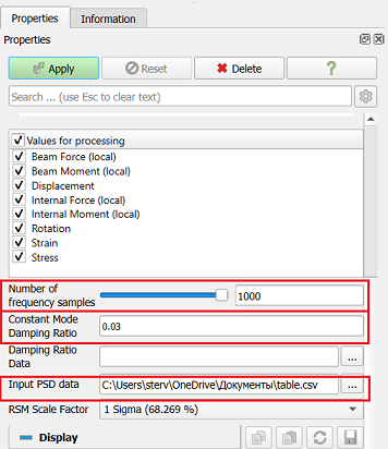
1. Select the point corresponding to vertex 2 (node ​​ID 2). Mainly menu, go to the tab Filters - Alphabetical - Random Vibration. In the properties panel that appears, click “Copy Active Selection”, then set the following options:

• Select the Number of frequency samples: 1000;

• Constant Mode Damping Ratio: 0.03;

• Specify the path of the CSV file generated at the beginning of the example, on your computer.

Click Apply.

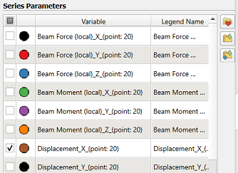
2. In the Series Parameters section, select only Displacement_X_(point: 20).

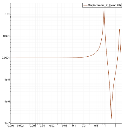
As a result, a graph of Displacement_X_(point: 20).

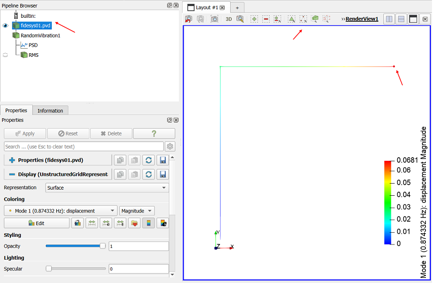
3. Next, in the Pipeline Browser, select the original name of the pvd file (for example, in our version fidesys01.pvd) and select node 12 in accordance with point 1 (node ​​12 is located at the free end of the vertical beam).

4. Then in the Pipeline Browser you need to select the filter RandomVibration1, and in the Property tab, click “Copy Active Selection”. Click Apply.

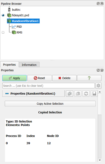
5. Next, in the Pipeline Browser, select the PSD subfilter and make active view with graphs (blue frame).

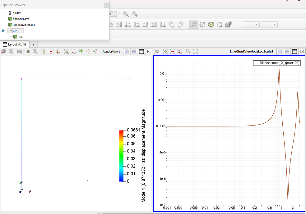
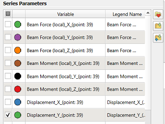
6. In the Series Parameters section, select only Displacement_Y_(point: 39).

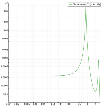
As a result, a graph of  Displacements_Y_(point: 39).

7. Then in the Pipeline Browser select the RMS subfilter and make active view with diagrams (blue frame).

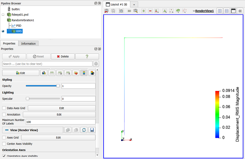
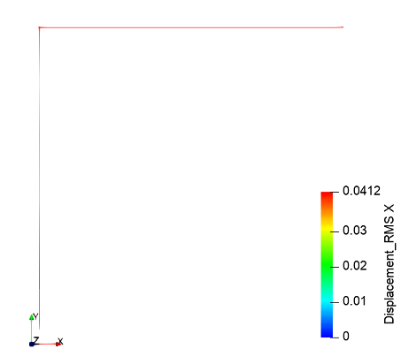
8. Next, on the top panel, from the first drop-down list, select Displacement_RMS, from the second – X.

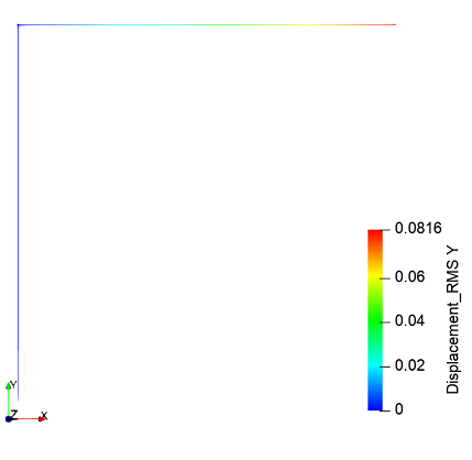
9. Display the calculation result data for the Y component.

Using Console Interface

Geometry creating, meshing, setting boundary conditions and materials can be performed using the console interface. Below is a link to the program code that allows you to perform the steps described above manual, you only need to specify the full path and name.

random_vibration