Search the documentation
Enter at least 2 characters
Enter at least 2 characters
 |
CAE Fidesys 9.0 Documentation |
An example of reducing a 3D problem for a body of rotation to a two-dimensional axisymmetric problem is considered. The problem of static loading of a truncated cone made of carbon steel is solved. The geometric model of the problem is shown in the figure below:
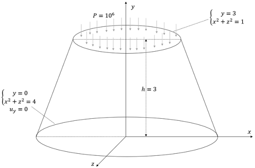
Fig.1 - An illustration of a three-dimensional problem statement
The body is a truncated cone made of carbon steel with a height of h = 3. The lower base is located on the Oxz plane, its center coincides with the center of coordinates. The radius of the lower base is 2, the radius of the upper base is 1. The axis of symmetry the cone coincides with the Y-axis. A pressure of 1e6 is applied to the upper base. The lower base is fixed along the Y axis. Important: both the geometry and the boundary conditions are symmetrical with respect to the Y axis! The two-dimensional equivalent of the illustration for the problem is presented below:
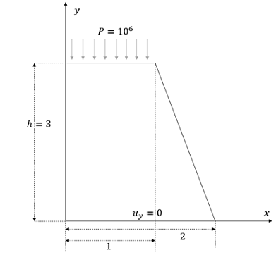
Fig.2 - An illustration of a two-dimensional axisymmetric problem statement
It is easy to see that by rotating the trapezoid in Fig. 2 around the Y axis, we get a truncated cone in Fig. 1.
At this point, we note that in an axisymmetric formulation, the location of the figure relative to the axis of symmetry is essential. Even with the usual displacement of all the elements of the problem in Fig. 2 by the same vector, the resulting figure will correspond to another three-dimensional problem. For example, if we shift all the elements of Fig. 2 to the right, then when rotating the figure around the Y axis, we get not a truncated cone from Fig. 1, but a hollow truncated cone.
1.Create a truncated cone.
On the command bar, select the module for constructing volume geometry (Mode - Geometry, Entity - Volume, Action - Create).
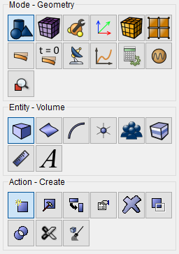
From the list of geometric primitives, select Cone.
Set the parameters:
Height: 3;
Top Radius: 1;
The shape of the base: Circular;
Radius: 2.
Click Apply.
2. Rotate the cone so that its axis of symmetry coincides with the Y axis.
On the command bar, select the module for constructing volume geometry (Mode - Geometry, Entity - Volume, Action - Transform).
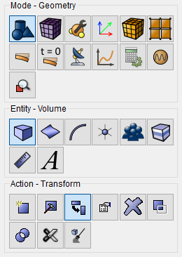
From the list of transforms, select Rotate.
Set the parameters:
Volume ID(s): 1;
Angle: -90;
Rotate About: Х-Axis.
Click Apply.
3. Leave only half of the truncated cone so that the cut surface lies in the XY plane.
On the command bar, select the module for constructing volume geometry (Mode — Geometry, Entity — Volume, Action — Webcut).
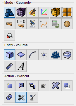
From the list, select Coordinate Plane.
Set the parameters:
Volume ID(s): 1;
With Plane: XY;
Offset Value: 0.
Click Apply.
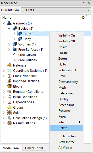
As a result, the original body in the object tree will be divided into two (Body 1 and Body 2). Delete Body 1.
To do this, right-click on Body 1 in the Model tree, and click in the pop-up menu Delete. As a result, only one half of the truncated cone will remain, that is, Body 2.
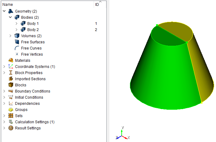
For a two-dimensional axisymmetric formulation of the problem, we are only interested in the resulting cut surface (Surface 8). The three-dimensional body itself should be removed. But when it is removed, the incision surface we need will also be removed. Therefore, you should copy it, getting a free surface.
4. Create a copy of the cut surface as a free surface.
On the command bar, select the module for constructing surface geometry (Mode — Geometry, Entity — Surface, Action — Create).
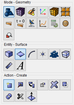
From the list of possible creation modes, select Copy and Transform.
Set the parameters:
Surface ID(s): 8;
Action: Move.
Leave the other parameter fields empty.
Click Apply.
As a result, a free surface was created — Surface 12 — coinciding with the surface of the incision, but not entering the original three-dimensional body.
5. Delete the remaining half of the three-dimensional body. To do this, hold down the Ctrl key, select Body 2 in the Model tree, and press in the context menu Delete. As a result, only free will remain Surface 12 (forming the Body 3). At the moment, it does not yet match the figure shown in Fig. 2.
6. Leave only the right half of the trapezoid so that the figure lies only in the area x ≥ 0.
On the command bar, select the module for constructing volume geometry (Mode — Geometry, Entity — Volume, Action — Webcut).
From the list, select Coordinate Plane.
Set the parameters:
Volume ID(s): 3;
With Plane: YZ;
Offset Value: 0.
Click Apply.
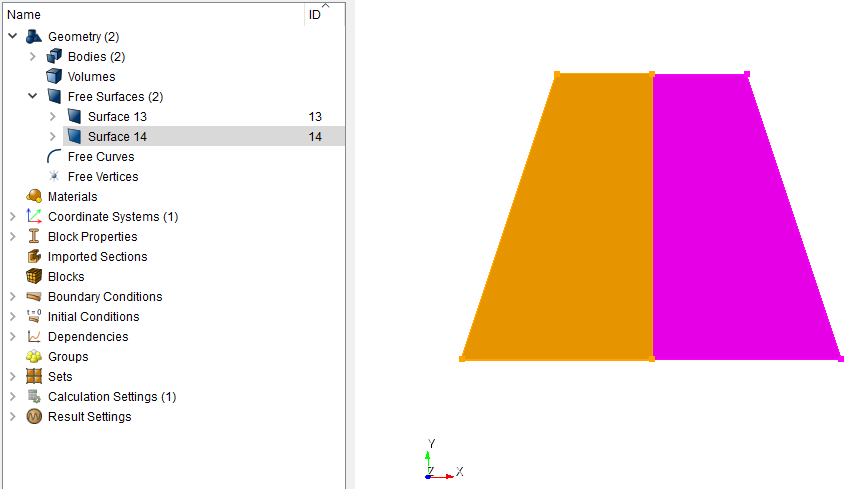
The surface 12 was divided into left (Surface 14) and right (Surface 13) halves. Remove the extra left half. To do this, right-click on in the Model tree Surface 14 and in the pop-up menu, press Delete. As a result, only one half of the trapezoid will remain — Surface 13.
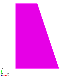
7. Since the task is now two-dimensional, to conveniently display the
shape in the top menu, click the button Front View -  .
.
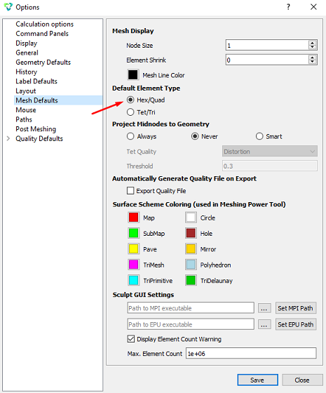
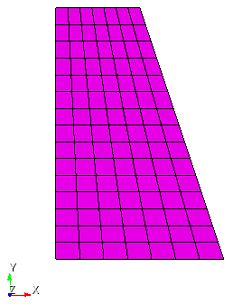
1. Make sure that in the settings of the main menu (Tools — Options — Mesh Defaults) selected Default Element Type Hex/Quad.
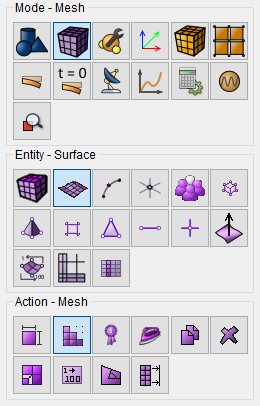
2. On the command bar, select the surface mesh module (Mode — Mesh, Entity – Surface, Action – Mesh).
Specify:
Select the mesh scheme: Automatically Calculate;
Select Surfaces: 13.
Click Apply Scheme.
Click Mesh.
1. In the command bar, select the module for specifying material properties (Mode - Material, Entity - Materials Management).

In the Manage materials window that opens, from the third column to the second, transfer the material "Steel".
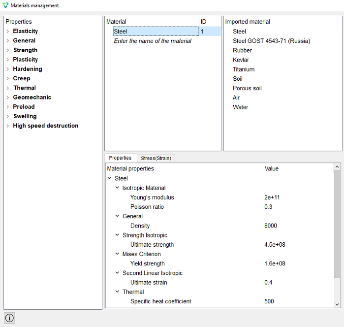
Click Apply.
Close the window Materials management.
2. Create a block.
On the command bar, select the block management module (Mode - Blocks, Entity - Block, Action - Add).

Set the parameters:
Block ID: 1;
Entity List: Surface;
Entity ID(s): 13.
Click Apply.
3. Set the block parameters.
On the command bar, select the block management module (Mode - Blocks, Entity - Block, Action - Block properties/parameters).

Set the parameters:
Block ID(s): 1;
Category: Plane;
Material: Steel;
Order: 1.
Click Apply.
1. Secure the bottom base of the trapezoid (which corresponds to the bottom base of the three-dimensional cone) along the Y axis.
On the command panel, select the boundary conditions module (Mode - Boundary Conditions, Entity - Displacement, Action - Create).
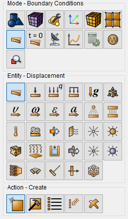
Set the parameters:
Entity List: Curve;
Entity ID(s): 20;
Degrees Of Freedom: Fix All.
Click Apply.
2. Apply pressure to the upper base of the trapezoid (which corresponds to the upper base of the three-dimensional cone).
On the command panel, select the boundary conditions module (Mode — Boundary Conditions, Entity — Pressure, Action — Create).
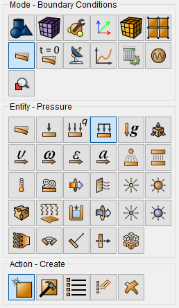
Set the parameters:
Entity List: Curve;
Entity ID(s): 21;
Value: 1e6.
Click Apply.
1. Set the type of problem you want to solve.
On the command panel, select the calculation settings mode (Mode - Calculation Settings, Calculation Settings - Static, Static - General).
Set the parameters:
Dimensions: 2D;
Plane state: Axisymmetric;
Model: Elasticity.
Click Apply.
Click Start Calculation.
2. In a pop-up window select a folder to save the result and enter the file name.
3. If the calculation is finished successfully, you will see a message in the Console: “Calculation finished successfully at "date time".
1. Open the file with the results. There are three ways to do that.
Click Ctrl+E.
From the main menu, select Calculation. Click Open results.
Select Results on Command Panel (Mode - Results). Click Open last result.

The FidesysViewer, window will appear, in which you can view the calculation results.
2. Display the component Uy of the displacement fields on the model. In the upper panel, select the calculation result data to display:
Representation Field: Displacement;
Representation Component: Y;
Representation Mode: Surface.
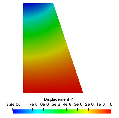
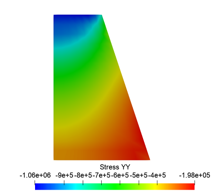
3. Display the voltage field component YY on the model. On the toolbar, set the following parameters:
Representation Field: Stress;
Representation Component: YY;
Representation Mode: Surface.
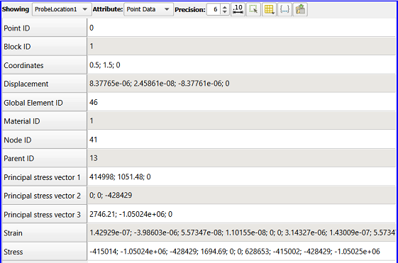
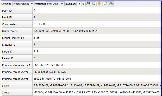
4. Output the calculation results for the point x = 0.5, y = 1.5, z = 0. On the command bar, select Filters - Alphabetical - Probe Location. In the properties tab, set the following parameters for this filter:
Center: (0.5, 1.5, 0);
Number Of Points: 1.
Click Apply.
Geometry creating, meshing, setting boundary conditions and materials can be performed using the console interface. Below is a link to the program code that allows you to perform the steps described above manual, you only need to specify the full path and name.
Let's compare the results of solving the problem with another method of solving it in Fidesys – in a three-dimensional formulation.
1. Enter the following commands in the command prompt:
reset
create frustum height 3 radius 2 top 1
rotate Volume 1  angle -90  about X include_merged
2. For the convenience of further analysis of the results, we will leave only a quarter of the three-dimensional cylinder.
Select volume geometry generation section on Command Panel (Mode — Geometry, Entity — Volume, Action — Webcut).
From the list, select Coordinate Plane.
Set the parameters:
Volume ID(s): 1;
With Plane: YZ;
Offset Value: 0.
Click Apply.
Then repeat the same action with the following parameters:
Volume ID(s): 1;
With Plane: XY;
Offset Value: 0.
In the Model tree, right-click on Body 1, and in the pop-up menu, click Delete. Also delete Body 2. As a result, only a quarter of the cone remains – Body 3.
1. Make sure that in the settings of the main menu (Tools — Options — Mesh Defaults) selected Default Element Type Hex/Quad.
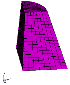
2. On the command panel, select (Mode — Mesh, Entity – Volume, Action – Mesh).
Specify:
Select the mesh scheme: Automatically Calculate;
Select Volumes: 3.
Click Apply Scheme.
Click Mesh.
1. On the command panel, select the mode for setting material properties (Mode - Material, Entity - Materials Management).
In the Manage materials window that opens, from the third column to the second, transfer the material "Steel".
Click Apply. Close the window Materials management.
2. Create a block.
On the command panel, select the mode for setting material properties (Mode - Blocks, Entity - Block, Action - Add).
Set the parameters:
Block ID: 1;
Entity List: Volume;
Entity ID(s): 3.
Click Apply.
3. Set the block parameters.
On the command panel, select the mode for setting material properties (Mode - Blocks, Entity - Block, Action - Block properties/parameters).
Set the parameters:
Block ID(s): 1;
Category: Solid;
Material: Steel;
Order: 1.
Click Apply.
1. Fix the lower base of the truncated cone along the Y axis.
On the command panel, select (Mode - Boundary Conditions, Entity - Displacement, Action - Create).
Set the parameters:
Entity List: Surface;
Entity ID(s): 18;
Degrees Of Freedom: Y.
Click Apply.
2. Fix the axis of the truncated cone along the Z axis.
Set the parameters:
Entity List: Surface;
Entity ID(s): 17;
Degrees Of Freedom: Z.
Click Apply.
3. Fix the axis of the truncated cone along the X axis.
Set the parameters:
Entity List: Surface;
Entity ID(s): 19;
Degrees Of Freedom: X.
Click Apply.
4. Apply pressure to the upper base of the truncated cone.
On the command panel select (Mode — Boundary Conditions, Entity — Pressure, Action — Create).
Set the parameters:
Entity List: Surface;
Entity ID(s): 20;
Value: 1e6.
Click Apply.
5. Apply the periodic condition to the cut surfaces of the truncated cone.
On the command panel select (Mode — Boundary Conditions, Entity — Periodic Condition, Action — Create).
Set the parameters:
Master Entity: Entity List: Surface;
Master Entity: Entity ID(s): 19;
Slave Entity: Entity List: Surface;
Slave Entity: Entity ID(s): 17;
Type of periodic condition: General;
Coordinate System: Global Cartesian;
Number of Sectors: 4.
Click Apply.
1. Set the type of problem you want to solve.
On the command bar, select the calculation settings module (Mode - Calculation Settings, Calculation Settings - Static, Static - General).
Set the parameters:
Dimensions: 3D;
Model: Elasticity.
Click Apply.
Click Start Calculation.
2. In a pop-up window select a folder to save the result and enter the file name.
3. In the case of a successful calculation, the console displays the message: Calculation finished successfully at "date" "time".
1. Open the file with the results. There are three ways to do that.
Click Ctrl+E.
From the main menu, select Calculation. Click Open Results.
Select Results on Command Panel (Mode - Results). Click Open results.
The FidesysViewer, window will appear, in which you can view the calculation results.
2. Display the Uy component of the displacement fields on the model. In the upper panel, select the data calculation results to display:
Representation Field: Displacement;
Representation Component: Y;
Representation Mode: Surface.
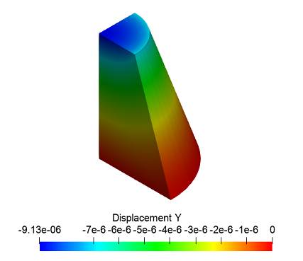
Note that due to the division of the cone into four parts and the periodic boundary condition, we can observe the section of the cone coinciding with a two-dimensional surface in the axisymmetric case.
3. Output the calculation results for the point x = 0.5, y = 1.5, z = 0.
On the command bar, select Filters - Alphabetical - Probe Location. In the properties tab, set the following parameters for this filter:
Center: (0.5, 1.5, 0);
Number Of Points: 1.
Click Apply.
Geometry creating, meshing, setting boundary conditions and materials can be performed using the console interface. Below is a link to the program code that allows you to perform the steps described above manual, you only need to specify the full path and name.