Search the documentation
Enter at least 2 characters
Enter at least 2 characters
 |
CAE Fidesys 9.0 Documentation |
To conduct the analysis, it is necessary to prepare a file in *.csv format. The file must contain a table, where the first column contains the values of the number of cycles, and the second column contains the values of the stresses. It is necessary to specify the column names:
This table is created as a CSV file and then imported into FidesysViewer (the image shows an example of setting up a table in Excel).
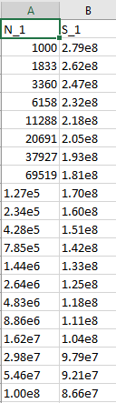
Note: Microsoft Excel can open a csv-file in this format:
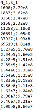
i.e. without breaking the file into columns and listing the file line values through a comma.
To separate the text in the lines by the corresponding columns, you need to put a comma in the list element separator settings of your operating system.
It is worth noting that if the settings are not changed, the file will not load correctly.
Download sample table.1. Create a brick.
On the command bar, select the module for constructing volume geometry (Mode — Geometry, Entity — Volume, Action — Create).
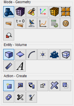
From the list of geometric primitives, select Brick.
Set the block dimensions:
X (width): 0.006;
Y (height): 0.012;
Z (depth): 0.25.
Click Apply.
1. Changing the mesh settings.
In order for the quadrilateral mesh to be built automatically, let's change the default settings. In the standard line, select Tools –Options.
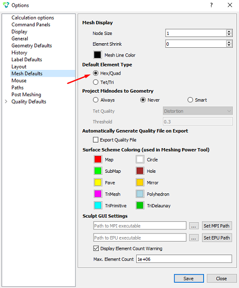
In the window that opens, in the left column, select Mesh Defaults. In the Element Type panel, by default, set Hex/Quad.
Click Save.
2. On the command bar, select the volume mesh module (Mode — Mesh, Entity — Volume, Action — Intervals).
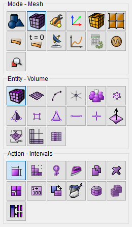
From the drop-down list, select: Automatic Sizing.
Select Volumes: all;
Auto Factor: 4.
Click Apply Size.
Click Mesh.
1. Specify the material.
In the command bar, select the module for specifying material properties (Mode — Material, Entity — Materials Management).

Specify the material name alum. Go to the Elasticity section and drag from the left column the Isotropic Material inscription to the Material Properties column. Specify the following parameters:
Young's modulus: 7.31e+10;
Poisson ratio: 0.
In the window on the left, go to the Strength/Isotropic Strength section and drag Ultimate strength to the Material Properties window. Enter the value:
Ultimate strength: 5.62e+08.
Next, go to the Plasticity/Mises Criterion. Drag Yield strength to the Material Properties window. Enter values:
Yield strength: 2e+08.
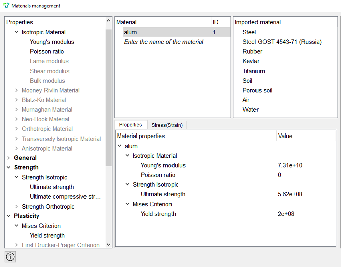
Click Apply.
Close the Material Management window.
2. Create a block of one material type.
On the command bar, select the block management module (Mode — Blocks, Entity — Block, Action — Add).

Set the following parameters:
Block ID: 1;
Entity List: Volume;
Entity ID(s) : 1.
Click Apply.
3. Set the block parameters.
On the command bar, select the block management module (Mode — Blocks, Entity — Block, Action — Block properties/parameters).

Set the following parameters:
Block ID(s): 1;
Category: Plane;
Material: alum;
Coordinate System: Global Cartesian;
Order: 1.
Click Apply.
1. Fix surface 2 in all directions.
On the command bar, select the boundary conditions module (Mode — Boundary Conditions, Entity — Displacement, Action — Create).
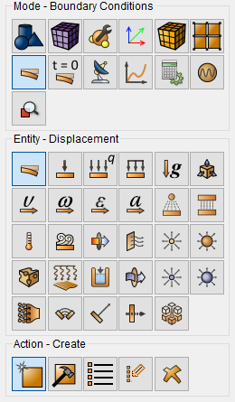
Set the following parameters:
Entity List: Surface;
Entity ID(s): 2;
Degrees of Freedom: Fix All.
Click Apply.
2. Set the distributed force.
On the command bar, select the boundary conditions module (Mode — Boundary Conditions, Entity — Distributed Force, Action — Create).
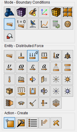
Set the following parameters:
Entity List: Surface;
Entity ID(s): 1;
Force Type: Equivalent Force;
Force: 50;
Moment: 0;
Direction Vector X: 0;
Direction Vector Y: -10;
Direction Vector Z: 0.
Click Apply.
1. Specify the type of problem to be solved.
On the command bar, select the calculation settings module (Mode — Calculation Settings, Calculation Settings — Static, Static — General).
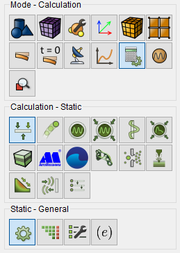
Select:
Dimensions: 3D;
Model: Elasticity.
Click Apply.
2. Set additional settings.
On the command bar, select the calculation settings module (Mode — Calculation Settings, Calculation Settings — Static, Static — Output Fields).
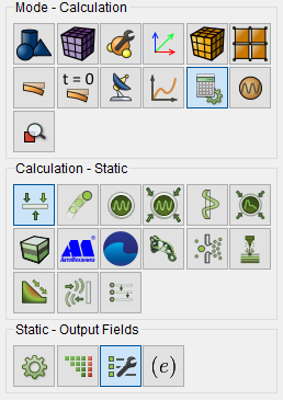
Check the box next to the parameters:
Click Apply.
Click Start Calculation.
3. In a pop-up window select a folder to save the result and enter the file name.
4. In the case of a successful calculation, the console displays the message: Calculation finished successfully at "date" "time".
1. Open the file with the results. There are three ways to do that.
Click Ctrl+E.
From the main menu, select Calculation. Click Open Results.
Select Results on Command Panel (Mode - Results). Click Open results.

The FidesysViewer window will appear, in which you can view the calculation results.
In the line bar, select Filters - Alphabetical - Fatigue.
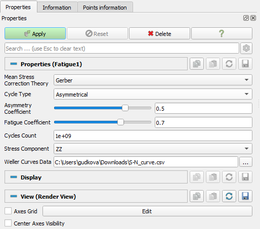
For the Fatigue filter, in the Properties tab, specify:
Array To Process: Stress;
Mean Stress Correction Theory: Gerber;
Cycle Type: Asymmetrical;
Asymmetry Coefficient: 0.5;
Fatigue Coefficient: 0.7;
Cycles Count: 1e+09;
Stress Component: ZZ;
Weller Curves Data: specify the path CSV file created at the beginning of the example on his computer.
Click Apply.
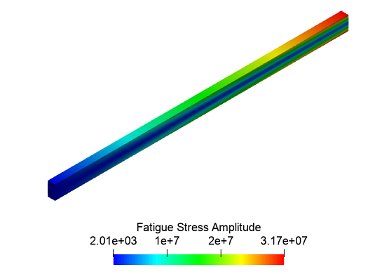
2. From the first drop-down list, select Fatigue, from the second - Stress Amplitude.
3. From the first drop-down list, select Fatigue, from the second - Life.
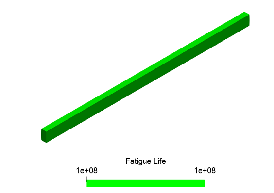
4. From the first drop-down list, select Fatigue, from the second - Damage.
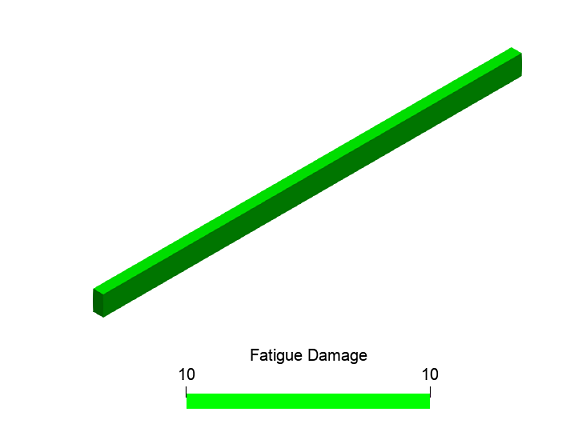
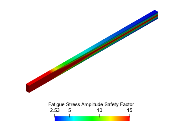
5. From the first drop-down list, select Fatigue, from the second - Stress Amplitude Safety Factor.
Geometry creating, meshing, setting boundary conditions and materials can be performed using the console interface. Below is a link to the program code that allows you to perform the steps described above manual, you only need to specify the full path and name.