Search the documentation
Enter at least 2 characters
Enter at least 2 characters
 |
CAE Fidesys 9.0 Documentation |
1. Create a brick.
On the command bar, select the module for constructing volume geometry (Mode - Geometry, Entity - Volume, Action - Create).
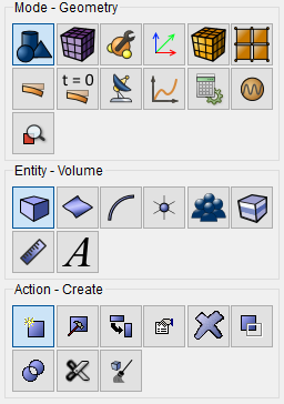
From the list of geometric primitives, select Brick.
Set the following parameters:
X (width): 432;
Y (height): 600;
Z (depth): 150.
Click Apply.
2. Move the brick.
On the command bar, select the module for constructing volume geometry (Mode - Geometry, Entity - Volume, Action - Transform).
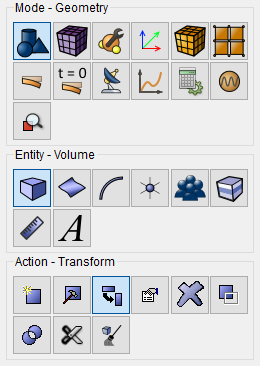
From the list select Move.
Set the following parameters:
Volume ID(s): 1;
Select Method: Distance;
X Distance: 216;
Y Distance: -300.
Click Apply.
3. On the command bar, select the module for constructing volume geometry (Mode - Geometry, Entity - Volume, Action - Create).
From the list of geometric primitives, select Brick.
Set the following parameters using APREPRO:
X (width): {12*13};
Y (height): {12*3};
Z (depth): 150.
Click Apply.
4. Move the brick №2.
On the command bar, select the module for constructing volume geometry (Mode - Geometry, Entity - Volume, Action - Transform).
From the list select Move.
Set the following parameters:
Volume ID(s): 2;
Select Method: Distance;
X Distance: 216;
Y Distance: -550.
Click Apply.
5. On the command bar, select the module for constructing volume geometry (Mode - Geometry, Entity - Volume, Action - Boolean).
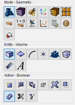
From the list select Subtract.
Set the following parameters:
A Volume ID(s): 1;
B Volume ID(s): 2;
Keep Originals;
Keep B.
Click Apply.
6. Creation of the cylinders.
But it is worth using APREPRO in case of creating several cylinders.
Enter the commands at the command line:
{i=0}
{n=3}
#{Loop(6)}
create Cylinder height 150 radius 6
move Volume {3+i} x {(5-2*i)*12+216} y -550 include_merged
#{i++}
#{EndLoop}
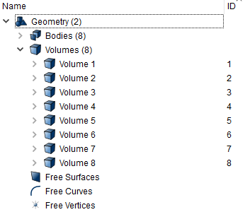
In the Model Tree on the left side you can see that 8 volumes have been created.
7. Subtract the cylinders from the brick.
On the command bar, select the module for constructing volume geometry (Mode - Geometry, Entity - Volume, Action - Boolean).
From the list select Subtract.
Set the following parameters:
A Volume ID(s): 2;
B Volume ID(s): 3 to 8.
Click Apply.
8. Imprint and merge all volumes.
On the command bar, select the module for constructing volume geometry (Mode - Geometry, Entity - Volume, Action – Imprint and Merge).
From the list select Imprint/Merge Volumes.
Set the following parameters:
Volume ID(s): all.
Click Apply.
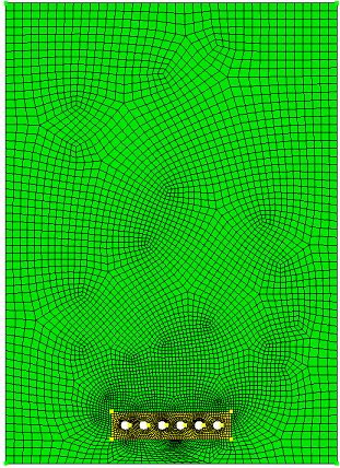
1. Mesh volume №2 using Geometry Adaptive function.
On the command bar, select the volume mesh module (Mode - Mesh, Entity - Volume, Action – Intervals).
From the list select Geometry Adaptive.
Set the following parameters:
Select Volumes: 2.
Click Apply Size.
2. Mesh all volumes using Sweep function.
On the command bar, select the volume mesh module (Mode - Mesh, Entity - Volume, Action – Mesh).
From the list select Sweep.
Set the following parameters:
Select Volumes: 1;
Auto Select Source and Target.
Click Apply Scheme.
Click Mesh.
3. Refine Mesh.
On the command bar, select the volume mesh module (Mode - Mesh, Entity - Volume, Action – Refine).
From the list select General Refinement.
Set the following parameters:
Volume ID(s): all;
Refinement Condition: Split Iterations;
Split Iterations: 2.
Click Apply.
In the command bar, select the module for specifying material properties (Mode - Material, Entity – Materials Management).

Drag material Soil from the column Imported material to Material.
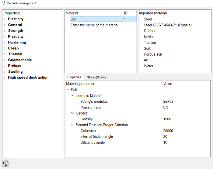
Click Apply.
Close the Materials management window.
1. On the command bar, select the block management module (Mode - Blocks, Entity - Block, Action - Add).

Set the following parameters:
Click Apply.
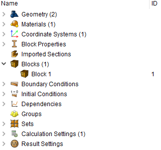
2. Set the block parameters.
On the command bar, select the block management module (Mode - Blocks, Entity - Block, Action - Block properties/parameters).

Set the following parameters:
Block ID(s): 1 or all;
Category: Solid;
Material: Soil;
Coordinate System: Global Cartesian;
Order: 2.
Click Apply.
1. Create gravity.
On the command panel, select the boundary conditions module (Mode - Boundary Conditions, Entity - Gravity, Action - Create).
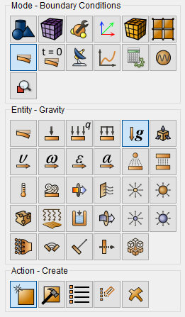
Set the following parameters:
Entity List: Global;
Directions: Y: -9.8.
Click Apply.
2. Fix surfaces 4 and 6 along the X-axis.
On the command panel, select the boundary conditions module (Mode - Boundary Conditions, Entity - Displacement, Action - Create).
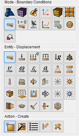
Set the following parameters:
Entity List: Surface;
Entity ID(s): 6 4;
Degrees Of Freedom: X-Translation Disp;
DOF Value: 0.
Click Apply.
3. Fix surface 3 in all degrees of freedom.
Set the following parameters:
Entity List: Surface;
Entity ID(s): 3;
Degrees Of Freedom: All;
DOF Value: 0.
Click Apply.
4. Fix surfaces 18, 44, 17, 43 along the Z-axis.
Set the following parameters:
Entity List: Surface;
Entity ID(s): 17 18 44 43;
Degrees Of Freedom: Z-Translation Disp;
DOF Value: 0.
Click Apply.
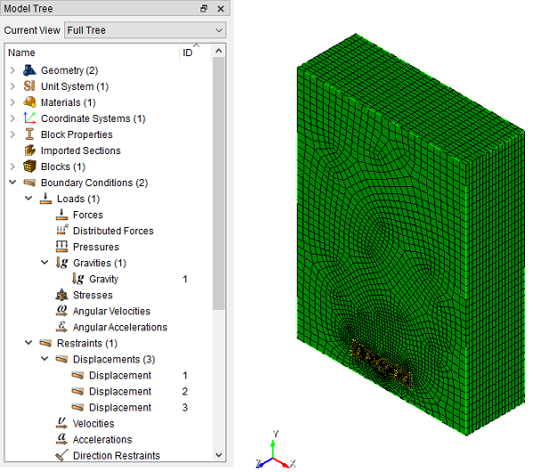
All boundary conditions can be viewed in the Model Tree on the left side.
1. Set the type of the problem to be solved.
On the command bar, select the calculation settings module (Mode — Calculation Settings, Calculation Settings — Static, Static — General).
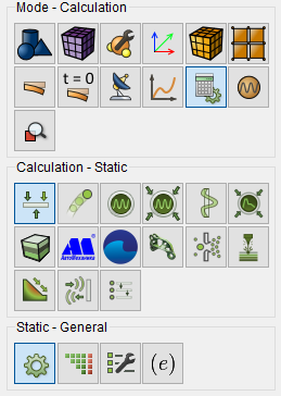
Select:
Dimensions: 3D;
Model: Elasticity.
Click Apply.
2. On the command bar, select the calculation settings module (Mode — Calculation Settings, Calculation Settings — Static, Static — Output Fields).
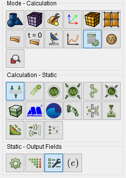
Select:
Output material properties;
Output Static or Preload intermediate results;
Output intermediate results: Every (substeps): 1.
Click Apply.
Click Start Calculation.
3. In the window that appears, select the directory in which the result will be saved, and enter the file name.
4. In the case of a successful calculation, the console displays the message: Calculation finished successfully at "date" "time".
1. Open the file with the results. There are three ways to do that.
Click Ctrl+E.
From the main menu, select Calculation. Click Open Results.
Select Results on Command Panel (Mode - Results). Click Open results.

The FidesysViewer window will appear, in which you can view the calculation results.
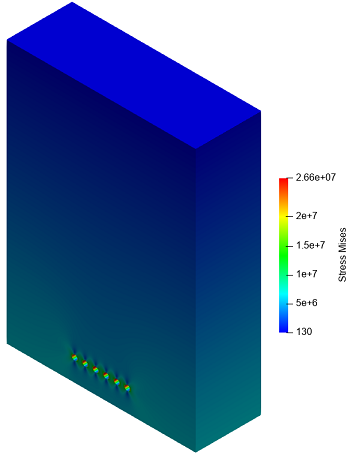
2. Select the Stress array on the panel:
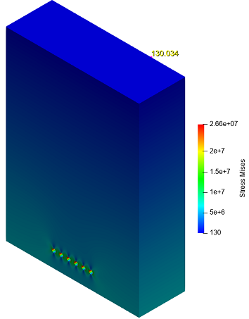
3. Click the min button in the working window to display the smallest value of von Mises stress:
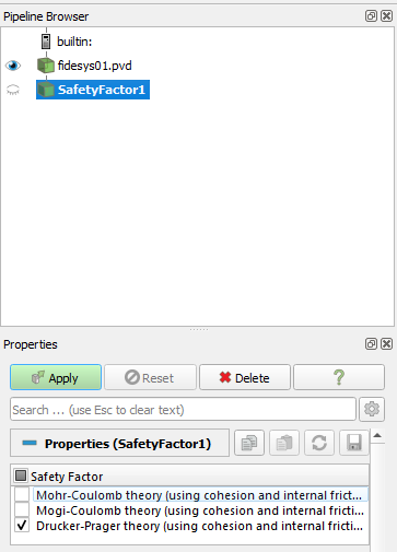
4. Go to Filters - Alphabetical. Select "Safety Factor" in the filters, check the theories of interest, in our case, it is Drucker-Prager theory (using cohesion and internal friction).
Click the Apply button for the filter.
After applying the filter, the following picture should be displayed:
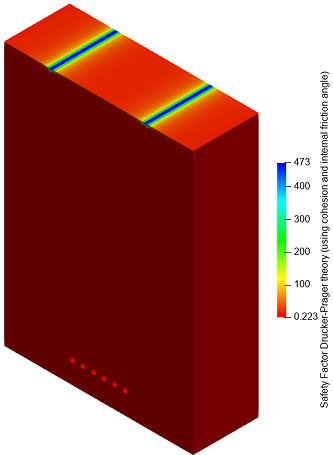
Click the max button in the work window to display the largest
value of the safety factor for the selected theory. Note that the smallest
value of von Mises stress corresponds to the largest value of the safety
factor.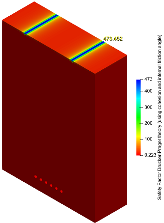
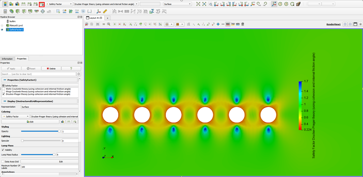
5. The purpose of this example is to study the safety factor around the workings. To do this, we rotate and enlarge the model as shown on the screen and rescale the results by the visible range by clicking on the corresponding button:
Geometry creating, meshing, setting boundary conditions and materials can be performed using the console interface. Below is a link to the program code that allows you to perform the steps described above manual, you only need to specify the full path and name.