Search the documentation
Enter at least 2 characters
Enter at least 2 characters
 |
CAE Fidesys 9.0 Documentation |
Consider the problem of stepwise loading of a plate with inclusion.
The properties of the material of which the inclusion consists change (aluminum is replaced by copper in the third step) in the process of loading,. The loading diagram is shown below.
1. Create rectangle.
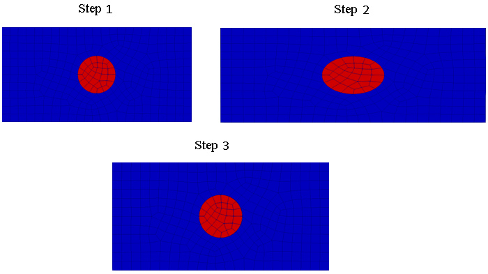
On the command bar, select the module for constructing surface geometry (Mode — Geometry, Entity — Surface, Action — Create).
From the list of geometric primitives, select Rectangle.
Set block sizes:
Width: 10;
Height: 5;
Location: ZPlane.
Click Apply.
2. Create a circular surface with a radius of 1.
From the list of geometric primitives, select Circle.
Set circle sizes:
Specify Circle Using: Radius;
Radius: 1;
Location: ZPlane.
Click Apply.
3. Subtract circle from rectangle.
On the command bar, select the module for constructing surface geometry (Mode — Geometry, Entity — Surface, Action — Boolean).
From the list of operations select Subtract.
Set the following parameters:
Surface ID(s): 1 (surfaces from which other surface will be subtracted);
Surface ID(s): 2 (amounts to be deducted);
Check the Keep Originals box and select Keep both (A and B).
Click Apply.
4. Delete the surface 1.
On the command bar, select the module for constructing surface geometry (Mode — Geometry, Entity — Surface, Action — Delete).
Surface ID(s): 1.
Click Apply.
5. Merge all curves.
On the command bar, select the module for constructing geometry (Mode — Geometry, Entity — Curve, Action - Merge).
From the list of possible transformations select Merge.
Set the parameters:
Curve ID(s): all.
Click Apply.
6. Use command compress all, for change surface numbering.
1. Create a rectangular finite element mesh.
On the command line, write set default element hex.
On the command bar, select the surface mesh module (Mode — Mesh, Entity — Surface, Action — Intervals).
Select the mesh scheme: Automatic Sizing;
Select Surfaces: all.
Auto Factor: 4 (move the slider to 4).
Click Apply Scheme.
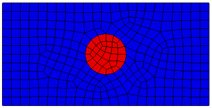
Click Mesh.
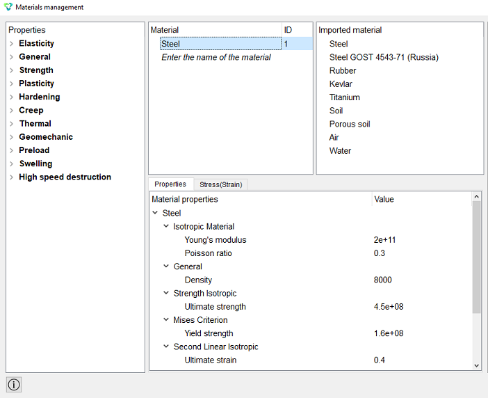
1. In the command bar, select the module for specifying material properties (Mode — Material, Entity — Materials Management).

1. Steel:
Young’s modulus E = 2e11;
Poisson ratio ν = 0.3.
2. Aluminum:
Young’s modulus E = 0.7e11;
Poisson ratio ν = 0.34.
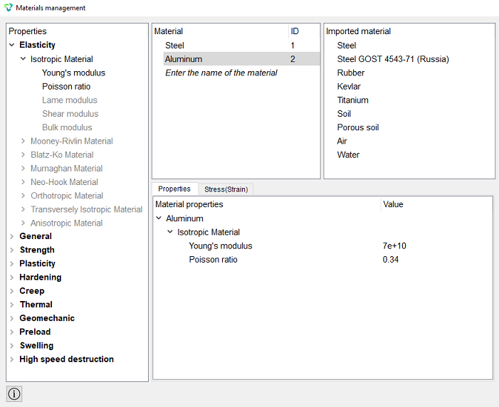
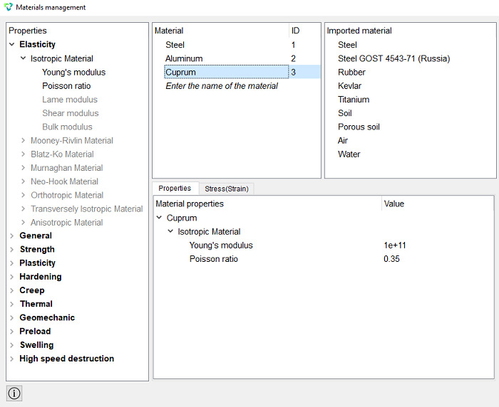
3. Cuprum:
Young’s modulus E = 1e11;
Poisson ratio ν = 0.35.
Click Apply.
Close the Materials management window.
2. Create 2 blocks Matrix and Inclusion.
On the command bar, select the block management module (Mode — Blocks, Entity — Block, Action — Add).

Set the following parameters:
Matrix:
Block ID: 1;
Entity List: Surface;
Entity ID(s): 2.
Inclusion:
Block ID: 2;
Entity List: Surface;
Entity ID(s): 1.
Click Apply.
3. Set the block № 1 parameters.
On the command bar, select the block management module (Mode - Blocks, Entity - Block, Action - Block properties/parameters).

Set the following parameters:
Block ID(s): 1;
Category: Solid;
Material: Steel;
Coordinate System: Global Cartesian;
Order: 2.
Click Apply.
4. Set the block № 2 parameters.
On the command bar, select the block management module (Mode - Blocks, Entity - Block, Action - Block properties/parameters).
Set the following parameters:
Block ID(s): 2;
Category: Solid;
Material: Aluminum;
Coordinate System: Global Cartesian;
Order: 2.
Click Apply.
1. Fix the left side at all directions.
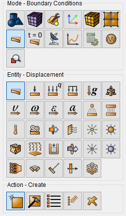
On the command panel, select the boundary conditions module (Mode — Boundary Conditions, Entity — Displacement, Action — Create).
Set the following parameters:
Entity List: Curve;
Entity ID(s): 3;
Degrees of Freedom: All.
Click Apply.
2. Fix the model along the Y axis.
On the command panel, select the boundary conditions module (Mode — Boundary Conditions, Entity — Displacement, Action — Create).
Set the following parameters:
Entity List: Curve;
Entity ID(s): 2 4;
Degrees of Freedom: Y-Translation Disp.
Click Apply.
3. Apply pressure to the right side curve.
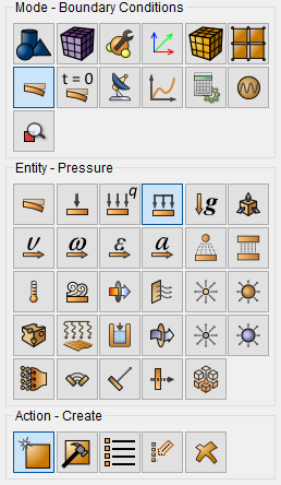
On the command panel, select the boundary conditions module (Mode — Boundary Conditions, Entity — Pressure, Action — Create).
Set the following parameters:
Pressure Entity List: Curve;
Entity ID(s): 5;
Magnitude Value: 1.
Click Apply.
4. Create table for pressure.
On the command panel, select the module for specifying Dependency BC (Mode - BC Dependency).
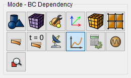
Click Pressure 1 and choose panel Table in the right side. Set the flag: Time and fill in the table as follows:
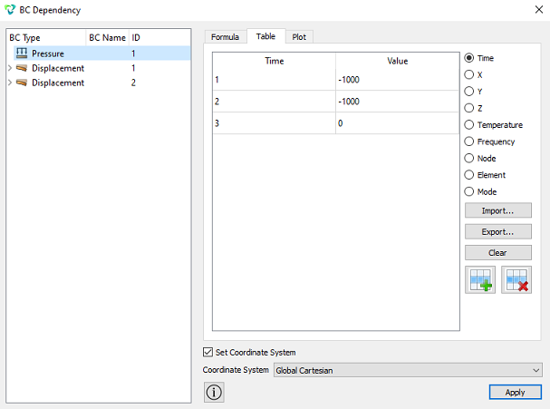
Click Apply.
1. Set the type of problem you want to solve.
On the command bar, select the calculation settings module (Mode — Calculation Settings, Calculation Settings — Static, Static — General).
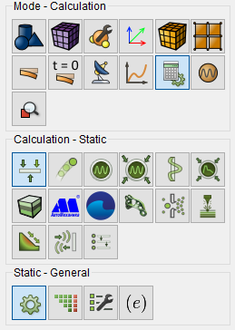
Set the following parameters:
Dimensions: 2D;
Plain state: Plane strain;
Model: Elasticity;
Set static load steps count: 3.
Click the button  opposite the field
with setting the number of loading steps. In the appeared Settings of
loading steps window select Set step materials for block 2.
opposite the field
with setting the number of loading steps. In the appeared Settings of
loading steps window select Set step materials for block 2.
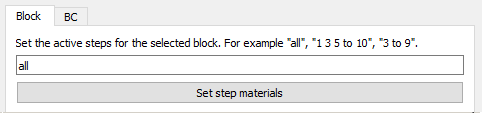
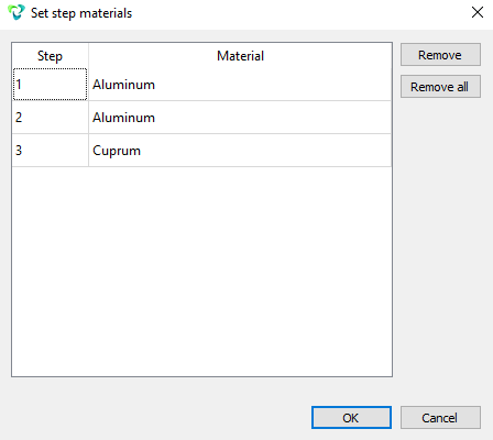
Next, fill in the table as follows:
Click OK.
Click Apply.
2. On the command bar, select the calculation settings module (Mode — Calculation Settings, Calculation Settings — Static, Static — Output Fields).
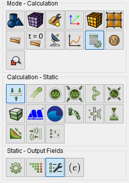
Check the box next to Output material properties.
Click Apply.
Click Start Calculation.0
2. In a pop-up window select a folder to save the result and enter the file name.
3. In the case of a successful calculation, the console displays the message: Calculation finished successfully at "date" "time".
1. Open the file with the results. There are three ways to do that.
Click Ctrl+E.
From the main menu, select Calculation. Click Open Results.
Select Results on Command Panel (Mode - Results). Click Open results.

The FidesysViewer window will appear, in which you can view the calculation results.
Select any node on the inclusion surface using the Select Points On tool.
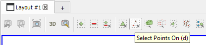
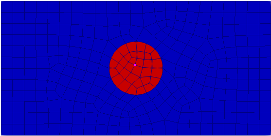
Plot a timeline for this point to make sure the change has occurred material properties during the calculation. Select Menu - Filters - Alphabetical - Plot Selection Over Time. Select Elastic Modules (Young's Modulus) as the field to display on the graph.
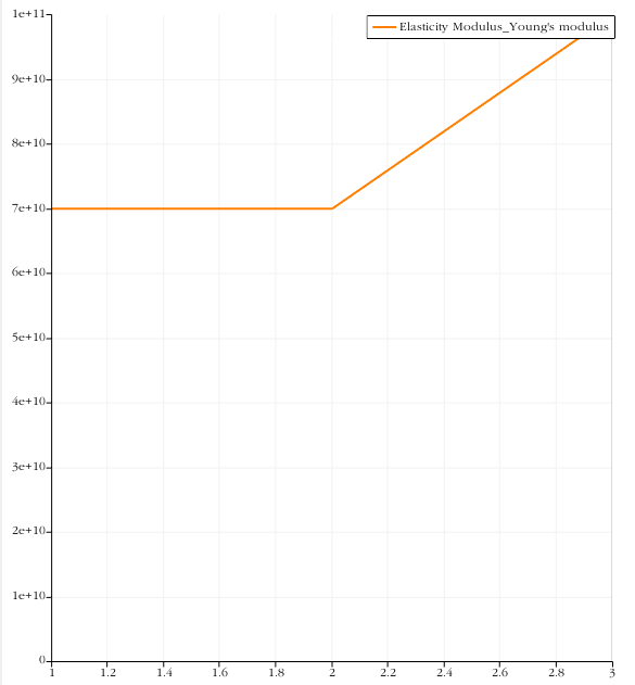
To rescale the vertical axis on the property page go to the Left axis range section and check the box next to Custom left axis range. Set the minimum value to 1e10.
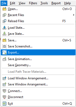
Save the resulting data to a .csv table. Go to Menu - File - Export....
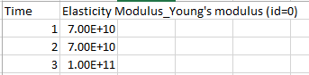
Save csv file, then open it.
Geometry creating, meshing, setting boundary conditions and materials can be performed using the console interface. Below is a link to the program code that allows you to perform the steps described above manual, you only need to specify the full path and name.