Periodic Conditions

Boundary condition "Periodic condition" binds the value the selected parameter (displacement, velocity, acceleration, temperature, pore pressure) of the two groups of nodes of the finite elements model by coupling equations in accordance with a certain law. BC can be applied to both geometric objects (surface,curve, vertex), and to other objects (side, edge of the element or a node). If it is applied to geometric objects, it will be applied to nodes belonging to the selected geometry.

Boundary condition "Periodic condition" allows you to all types of calculations (modal analysis, static loading - linear and taking into account plasticity, step-by-step loading, nonlinear dynamics) on segment of the object model.

The use of such a BC is advisable if the model is axisymmetric and it is possible to allocate a segment in it, by sequential copying of which an initial complete model can be obtained around the axis of symmetry. Either the model represents a periodicity cell.

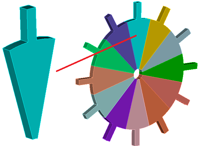
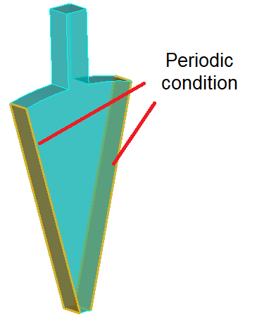
To apply this BC, it is necessary to attach it to two sides, which would be in contact with other segments in the case of a complete model.

The application of the BC to a flat or shell model is performed in the same way in a way, only it is no longer applied to surfaces, but to two curves bounding a flat segment.

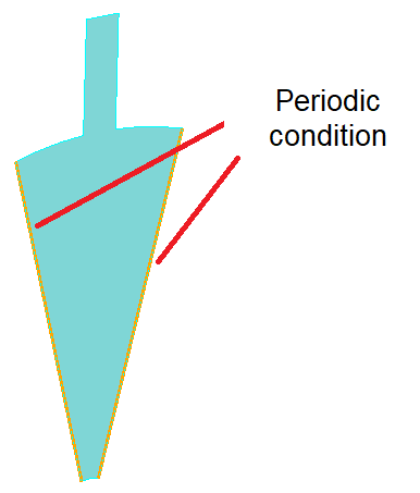
An example of the application of the BC Periodic condition.

The user can set periodic boundary conditions that apply to objects of dimensions 0D, 1D and 2D. To do this, follow these steps:

On the Command Bar, select Mode - Boundary Conditions.
Select Entity - Periodic Condition.
Depending on the situation, choose Action - Create or Action - Modify.
Using graphical user interface elements set the identifier (ID) of the Main and Secondary entities, specify the type of connection - General, Displacement, Speed, Acceleration, Temperature, Pore pressure.
Select a coordinate system (see below).
Specify the number of sectors (to display full model).
Click Apply.

Important: For calculations taking into account cyclic symmetry it will be sufficient to specify a Cartesian system coordinates. In fact, for the correct calculation, the direction of the Z axis and the origin point are necessary.

To display the complete model in the postprocessor, it is necessary when setting a periodic boundary condition, specify the number of sectors, and then, when starting the calculation, go to the Output Field settings and put check the box next to the option Output a complete model (for periodic BC).

The corresponding commands entered in the command prompt window, have the form:

create periodic [[id] ] [name ] master {surface|curve|face|tri|edge|sideset|vertex|node|nodeset} {[[id] {[] [ to ]}...] [all] [except {[] [ to ]}...]} slave {surface|curve|face|tri|edge|sideset|vertex|node|nodeset} {[[id] {[] [ to ]}...] [all] [except {[] [ to ]}...]} {general|displacement|velocity|acceleration|temperature|porepresure} [cs {|}] [step {[[id] {[] [ to ]}...] [all] [except {[] [ to ]}...]}] [{[value] |formula |table

modify periodic {[[id] {[] [ to ]}...] [] [all] [except {[] [ to ]}...]} [name ] [master {surface|curve|face|tri|edge|sideset|vertex|node|nodeset} {[[id] {[] [ to ]}...] [all] [except {[] [ to ]}...]}] [slave {surface|curve|face|tri|edge|sideset|vertex|node|nodeset} {[[id] {[] [ to ]}...] [all] [except {[] [ to ]}...]}] {general|displacement|velocity|acceleration|temperature|porepresure} [cs {|}] [step {[[id] {[] [ to ]}...] [all] [except {[] [ to ]}...]}] [{[value] |formula |table}]

The parameters (options) of these commands are described below.

Parameters

The key parameters are the numbers of the main entities (master) and side entities (slave) objects, selected condition parameter - displacement, velocity, acceleration, temperature, pore pressure, as well as the value for the selected condition parameter.

By default, the General condition parameter is set.