Search the documentation
Enter at least 2 characters
Enter at least 2 characters
 |
CAE Fidesys 9.0 Documentation |
There is some initial design area. The locations of the constraints and the location of the load are known. The problem is to remove from the area all unstressed and low-stressed material (all areas where the stresses are less than the specified value).
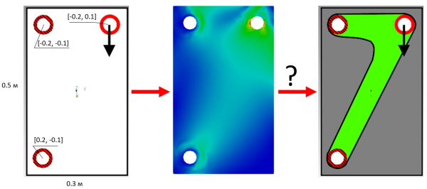
It is also necessary to build a 3D model suitable for subsequent additive manufacturing based on the result (optimized topology).
1. Create a rectangle.
On the command bar, select the module for constructing surface geometry (Mode — Geometry, Entity — Surface, Action — Create).
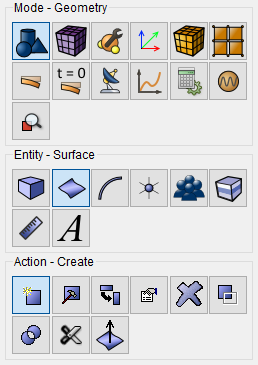
From the list of geometric primitives, select Rectangle.
Set the following parameters:
Width: 0.5;
Heigtht: 0.3;
ZPlane.
Click Apply.
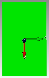
Rectangle will be created as on figure below.
2. Next, it is need to create 3 identical circles, which will allow you to set the boundaries of the unchangeable areas of future places of boundary conditions.
On the command bar, select the module for constructing surface geometry (Mode — Geometry, Entity — Surface, Action — Create).
From the list of geometric primitives, select Circle.
Set the following parameters:
Radius;
Radius: 0.03;
ZPlane.
Click Apply.
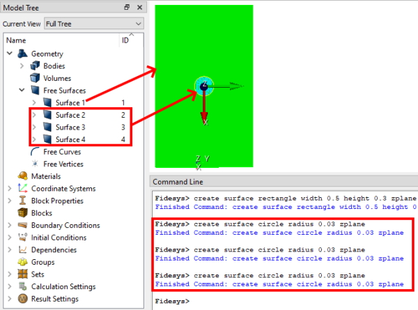
Repeat this procedure 2 more times, after which the following result can be seen.
3. Move the circles to the locations of the future areas of boundary conditions and loads.
On the command bar, select the module for constructing surface geometry (Mode — Geometry, Entity — Surface, Action — Transform).
From the list of actions, select Move.
Set the following parameters:
Surface ID(s): 2;
Distance;
Х Distance: 0.2;
Y Distance: -0.1;
Z Distance: 0.
Click Apply.
The selected circle will move to the specified distance.
4. Then repeat this procedure 2 more times with other values in the fields.
For surface 3, set the following parameters:
Surface ID(s): 3;
Distance;
Х Distance: -0.2;
Y Distance: -0.1;
Z Distance: 0;
Click Apply.
5. For surface 4, set the following parameters:
Surface ID(s): 4;
Distance;
Х Distance: -0.2;
Y Distance: 0.1;
Z Distance: 0.
Click Apply.
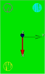
As a result, the following will be observed on the screen.
6. Then subtract the circles (surfaces 2, 3, and 4) from the rectangle (surface 1).
On the command bar, select the module for constructing surface geometry (Mode — Geometry, Entity — Surface, Action — Boolean).
From the list of actions, select Subtract.
Set the following parameters:
А Surface ID(s): 1;
B Surface ID(s): 2 3 4.
Click Apply.
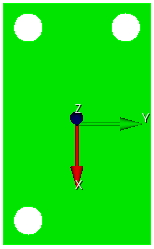
The result of these actions will be a surface with three holes, as shown in the figure below.
7. Then it is need to create 3 circles again, as it was done above.
On the command bar, select the module for constructing surface geometry (Mode — Geometry, Entity — Surface, Action — Create).
From the list of geometric primitives, select Circle.
Set the following parameters:
Radius;
Radius: 0.03;
ZPlane.
Click Apply.
And repeat this procedure again 2 more times.
8. Then move the created circles again. However, the new circles will have different surface numbers - 6, 7, and 8.
On the command bar, select the module for constructing surface geometry (Mode — Geometry, Entity — Surface, Action — Transform).
From the list of actions, select Move.
Set the following parameters:
Surface ID(s): 6;
Distance;
Х Distance: 0.2;
Y Distance: -0.1;
Z Distance: 0.
Click Apply.
Then repeat this procedure 2 more times with other values in the fields.
For surface 7, set the following parameters:
Surface ID(s): 7;
Distance;
Х Distance: -0.2;
Y Distance: -0.1;
Z Distance: 0.
Click Apply.
For surface 8, set the following parameters:
Surface ID(s): 8;
Distance;
Х Distance: -0.2;
Y Distance: 0.1;
Z Distance: 0.
Click Apply.
As a result, the following will be observed on the screen.
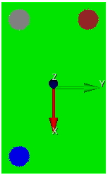
Create and move 3 more circles with a smaller radius in the same way.
On the command bar, select the module for constructing surface geometry (Mode — Geometry, Entity — Surface, Action — Create).
From the list of geometric primitives, select Circle.
Set the following parameters:
Radius;
Radius: 0.02;
ZPlane.
Click Apply.
Repeat this procedure 2 more times.
Then move the new circles (surfaces 9, 10 and 11) in the same way as the previous ones.
On the command bar, select the module for constructing surface geometry (Mode — Geometry, Entity — Surface, Action — Transform).
From the list of actions, select Move.
Set the following parameters:
Surface ID(s): 9;
Distance;
Х Distance: 0.2;
Y Distance: -0.1;
Z Distance: 0.
Click Apply.
The selected circle will move to the specified distance.
Then repeat this procedure 2 more times with other values in the fields.
For surface 10, set the following parameters:
Surface ID(s): 10;
Distance;
Х Distance: -0.2;
Y Distance: -0.1;
Z Distance: 0.
Click Apply.
For surface 11, set the following parameters:
Surface ID(s): 11;
Distance;
Х Distance: -0.2;
Y Distance: 0.1;
Z Distance: 0.
Click Apply.
As a result, the following will be observed on the screen.
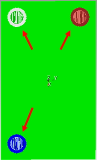
The next step is to "subtract" the surface of the small circles from the surfaces of the large circles.
On the command bar, select the module for constructing surface geometry (Mode — Geometry, Entity — Surface, Action — Boolean).
From the list of actions, select Subtract.
Set the following parameters:
А Surface ID(s): 7;
B Surface ID(s): 10.
Click Apply.
Then the following parameters:
А Surface ID(s): 8;
B Surface ID(s): 11;
Click Apply.
And the following parameters:
А Surface ID(s): 6;
B Surface ID(s): 9.
Click Apply.
The result of the actions performed is shown in the figure below.
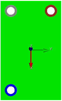
At the moment, all surfaces are unconnected and, when trying to create a mesh, the nodes on the boundaries of the surfaces will not join. In order to be able to build a suitable mesh, it is necessary to merge the lines at the joints of the surfaces.
On the command bar, select the module for constructing geometry (Mode — Geometry, Entity — Curve, Action — Merge).
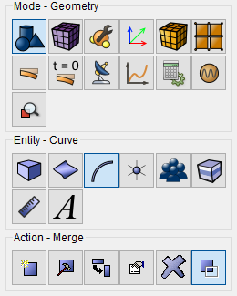
From the list of actions, select Merge.
Curve ID(s): all.
Click Apply.
1. Create a mesh.
On the command bar, select the surface mesh module (Mode — Mesh, Entity — Surface, Action — Intervals).
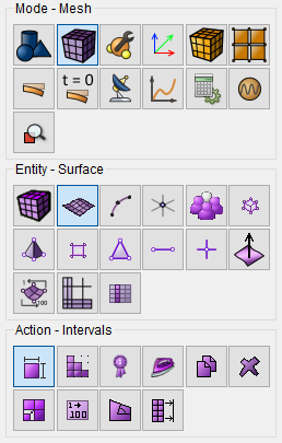
Select Approximate Size.
Set the following parameters:
Select Surfaces: all;
Approximate Size: 0.005.
Click Apply.
Click Mesh.
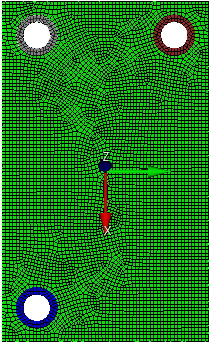
The result is shown in the figure below.
1. Create the material.
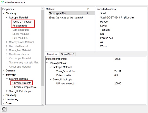
In the command bar, select the module for specifying material properties (Mode — Material, Entity — Materials Management). After that, the material management window will open, where you need to enter a name for the material that will be used.

After you have set the name (in this case, Topological Mat), you need to expand the property tree in the Elasticity - Isotropic Material branch and drag, holding down the left mouse button, the Young's Modulus and Poisson Ratio from the property tree to the lower right area.
In the same way, it is need to transfer the Ultimate strength from the Strength - Strength Isotropic branch.
Then set the values as in the example below.
Click Apply.
Close the Materials management window.
The next step is to create a block to pass properties to the surfaces.
2. Create a block.
On the command bar, select the block management module (Mode — Blocks, Entity — Block, Action — Add).

Select Surface in the list of possible operations.
Set the following parameters:
Block ID: all;
Entity list: Surface;
Entity ID(s): all.
Click Apply.
On the command bar, select the block management module (Mode — Blocks,
Entity — Block, Action — Block properties/parameters).

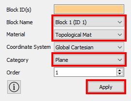
Set the following parameters:
Block Name: Block 1 (ID 1);
Category: Plane;
Material: Topological Mat;
Coordinate System: Global Cartesian;
Order: 1.
Click Apply.
1. Create boundary conditions.
On the command panel, select the boundary conditions module (Mode —
Boundary Conditions, Entity — Displacement, Action — Create).
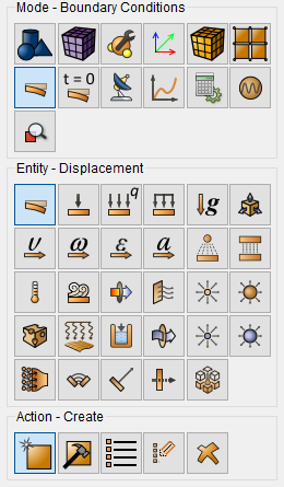
Set the following parameters:
Entity List: Surface;
Entity ID(s): 12 14;
Degrees Of Freedom: All.
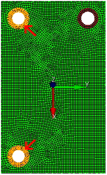
Click Apply.
Thus, not only were the boundary conditions created, but the regions of interest that must be preserved from the material removal algorithm were also "protected". This is the first way to "protect" immutable areas.
Apply the load.
2. On the command panel, select the boundary conditions module (Mode
— Boundary Conditions, Entity — Force, Action — Create).
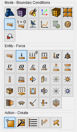
Set the following parameters:
Force Entity List: Curve;
Entity ID(s): 18;
Force: 100;
Direction X: 1 0 0.
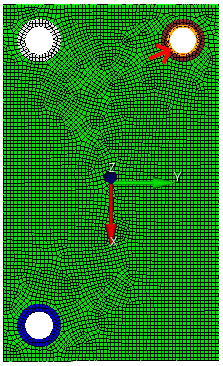
Click Apply.
Now it is necessary to "protect" the circular surface around the load application zone from the algorithm. To do this, a light load must be applied to the surface, which "protects" the surface without affecting the results. This is the second way to "protect" immutable areas.
3. On the command panel, select the boundary conditions module (Mode
— Boundary Conditions, Entity — Force, Action — Create).
Set the following parameters:
Force Entity List: Surface;
Entity ID(s): 13;
Force: 1e-6;
Direction X: 1 0 0.
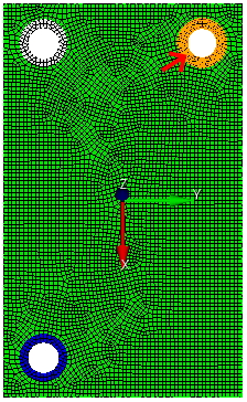
Click Apply.
1. Set the calculation settings.
Select calculation setting section on Command Panel (Mode — Calculation Settings, Calculation settings — Static, Static — General).
Dimensions: 2D.
Click Apply.
Click Start Calculation.
2. In the window that appears, select the directory in which the result will be saved and enter the file name.
3. In the case of a successful calculation, the console displays the message: Calculation finished successfully at "date" "time".
To view the results, go to the FidesysViewer postprocessor. To do this,
you need to go to (Mode - Results) and click Open last result.

Results of static calculation. Von Mises stresses.
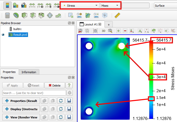
When analyzing the stress distribution, it is necessary to select the stress value that will be specified as the Ultimate strength in the calculation of topological optimization.
If you set the maximum value of the stresses in the structure as the Ultimate strength (in this example, 56400), then the optimization algorithm over-optimizes the structure, trying to remove from it almost everything except the zones protected by boundary conditions and loads (this problem is especially relevant for structures in which have zones with stress concentrators, where the stress values are orders of magnitude greater than the values in the main body). If you set the tensile strength too low (for example 5000), the algorithm will leave most of the material in place.
The algorithm tries to keep all zones where stresses are equal to or greater than the value specified as Ultimate strength.
Examples of the results of the calculation of topological optimization depending on the values of the Ultimate strength at step 20 (before the onset of the second stage - the last 1 step - thickening near the zones of boundary conditions and loads) of the calculation are shown in the figure below.
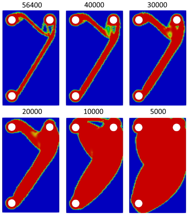
As an Ultimate strength for calculating topological optimization, it is necessary to select the highest values of stresses acting in the main body of the material (or on the most extensive area), but not more than the values of admissible stresses, if data for the structure are available. In this example, this value can be selected in the range from 10,000 to 30,000 (depending on the desired volume of material to be removed).
1. Set a new value for the Ultimate strength.
In this example, the value for Ultimate strength will be set to 20000.
On the command panel, select (Mode — Material, Entity — Materials Management).
Set the Ultimate strength value: 20000.
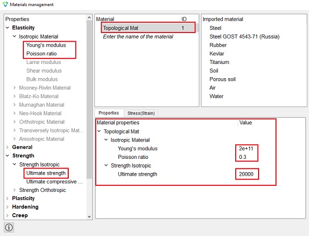
Then click Apply and then X in the upper right corner
of the Material Management panel.
2. Topological optimization calculation
On the command bar, select the calculation settings module (Mode — Calculation Settings, Calculation Settings — Topological Optimization).
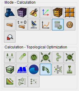
Set the following parameters:
Dimension: 2D;
Optimization iterations: 20;
Thickening iterations: 5.
Click Apply.
Click Start Calculation.
In the window that opens, select the location to save the results and the
file name. Then click Save.
Calculation starts.
When the calculation is completed, the following message will appear on the Command Line. After that, you can proceed to viewing the results.

To view the results, go to the FidesysViewer postprocessor. To do this,
you need to go to (Mode - Results) and click Open last result.
In the FidesysViewer window that opens, apply the Threshold
filter (Filters - Alphabetical - Threshold).
Then select step 20, select the input array Elasticity Modulus,
check the Only cells whose point values are within the range box
and click Apply.
Next, you need to move the slider of the minimum value of the modulus of
elasticity to a value of the order of 2e+9, (slider of the maximum
to 2e+11) and click Apply.
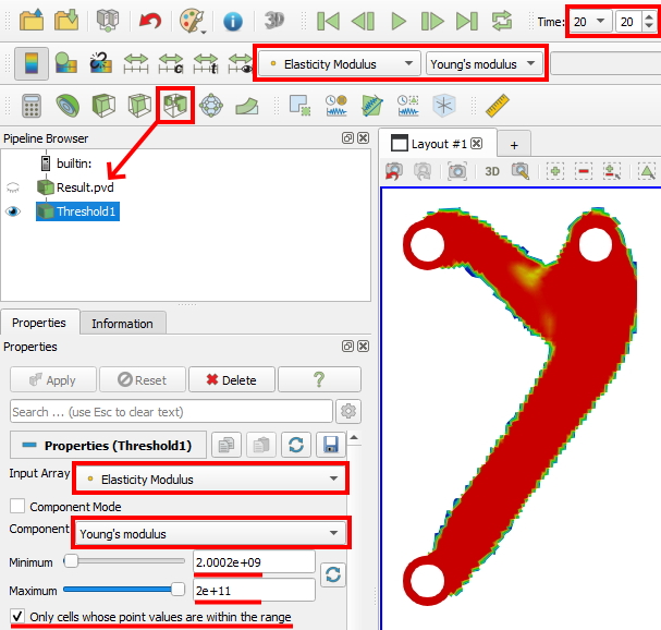
If everything was done correctly, then in the model window you will see the result - a topologically optimized shape. Then it can be exported in a format that able to import back into preprocessor.
Go to File — Save...
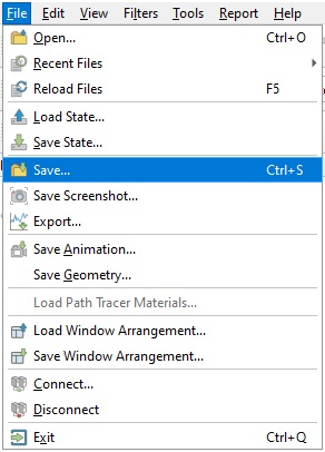
Select the save location and format .e and click OK.
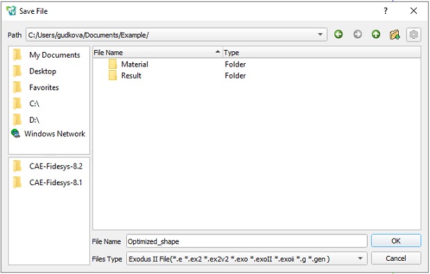
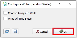
In the window that opens, click OK.
1. Open preprocessor.
Delete the surface mesh.
On the command panel, select (Mode — Mesh, Entity — Surface, Action — Delete).
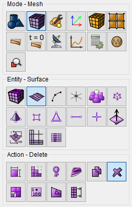
Fill the field Surface ID(s) with all.
Click Apply.
2. Import model.
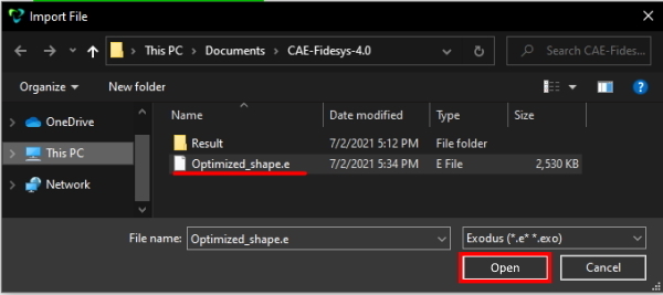
Go to menu File->Import.
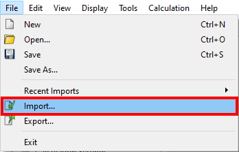
In the window that opens, find the file with extension .е, select it and click Open.
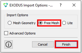
In next window that opens, select Free mesh and click Finish.
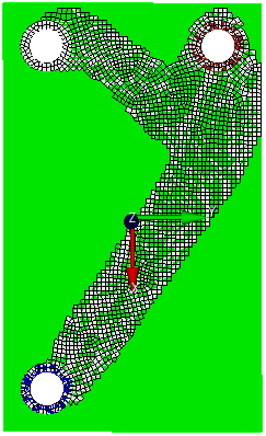
If everything was done correctly, you will see the shape of the optimized topology inside the geometry model.
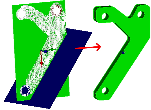
You can now edit the geometry to fit the shape of the optimized topology.
3. Remove unnecessary topology.
After the model has been edited and the topology shape is no longer needed, it must be deleted.
On the command panel, select (Mode — Mesh, Entity — Quad, Action — Delete).
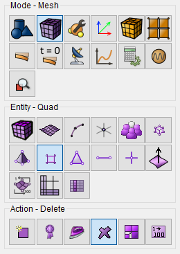
Fill the field Quad ID(s) with all.
Click Apply.
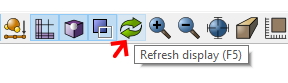
Then click on Refresh display button.
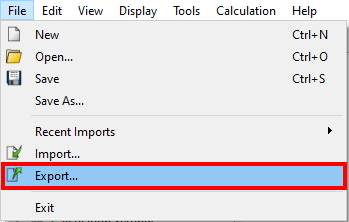
Go to menu File -> Export....
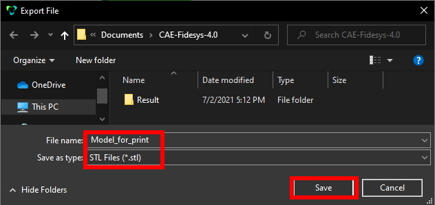
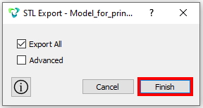
In the window that opens, select .stl extension and enter a name of file.
Click Save.
In next window click Finish.
Geometry creating, meshing, setting boundary conditions and materials can be performed using the console interface. Below is a link to the program code that allows you to perform the steps described above manual, you only need to specify the full path and name.