Search the documentation
Enter at least 2 characters
Enter at least 2 characters
 |
CAE Fidesys 9.0 Documentation |
The dynamic problem of thermal conductivity is solved taking into account a moving heat source and phase transitions (melting, evaporation, solidification). The physico-mathematical model of the process is formulated in the form of a nonlinear parabolic partial differential equation with respect to enthalpy. The defining equation is solved numerically by an implicit finite-volume scheme on a rectangular computational grid; at each time step, the SLAE is solved using a matrix-free implementation of the iterative conjugate gradient method.
1. Create the material.
In the command bar, select the module for specifying material properties (Mode - Material, Entity - Material Management).

Specify the name of the material Material 1.
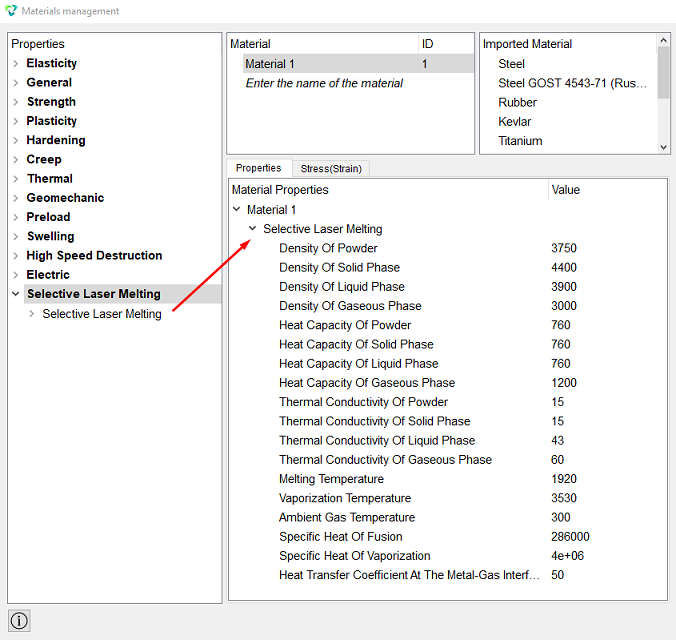
Drag the label Selective Laser Melting from the left column to the Material Properties column.
Set the following parameters:
Density Of Powder 3750;
Density Of Solid Phase 4400;
Density Of Liquid Phase 3900;
Density Of Gaseous Phase 3000;
Heat Capacity Of Powder 760;
Heat Capacity Of Solid Phase 760;
Heat Capacit Of Liquid Phase 760;
Heat Capacity Of Gaseous Phase 1200;
Thermal Conductivity Of Powder 15;
Thermal Conductivity Of Solid Phase 15;
Thermal Conductivity Of Liquid Phase 43;
Thermal Conductivity Of Gaseous Phase 60;
Melting Temperature 1920;
Vaporization Temperature 3530;
Ambient Gas Temperature 300;
Specific Heat Of Fusion 286000;
Specific Heat Of Vaporization 4e+06;
Heat Transfer Coefficient At The Metal-Gas Interface 50.
Click Apply.
Close the window Materials management.
1. Set the parameters for the laser calculation.
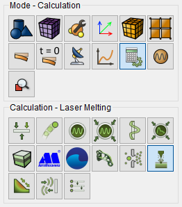
On the command bar, select the calculation settings module (Mode — Calculation, Calculation — Laser Melting).
Set the following values:
Model:
Material: Material 1;
Mesh Spacing: 5e-06;
Elements Along X: 130;
Elements Along Y: 80;
Elements Along Z: 50;
Powder Elements Along Z: 12.
Laser Parameters:
Power: 50;
Spot Radius: 4e-05;
Trajectory File: file
The format of the csv-file with the trajectory has the following structure:
Strings of the form 'x y t s', where x is the x‑coordinate (a floating‑point number), y is the y‑coordinate (a floating‑point number), t is the time (a floating‑point number), and s is an integer indicator that can take the values 0, 1, or 2.
The time stamps t must increase. Between two time stamps, the laser position is interpolated linearly based on the neighboring (x, y) values.
Indicator s = 0 is interpreted as “do nothing.” Indicator s = 1 is interpreted as “when this step is reached, cool everything in a single jump to T_ext” (this is required to speed up the calculation, since the alternative is to solve the cooling problem). Indicator s = 2 is interpreted as “when this step is reached, cool everything in a single jump to T_ext and ‘add a new layer of powder on top’; the grid size remains unchanged, and the old cells are shifted down.”
Simulation Parameters:
Max Time: 0.005;
Time Step: 2.5e-05;
Steps Count: 200;
Max Iterations: 50;
Tolerance: 0.0001;
Save Every (Steps): 10.
Click Apply.
Click Start Calculation.
2. In the window that appears, select the directory in which the result will be saved, and enter the file name.
3. In the case of a successful calculation, the console displays the message: Calculation finished successfully at "date" "time".
1. Open the file with the results. There are three ways to do that.
Click Ctrl+E.
From the main menu, select Calculation. Click Open Results.
Select Results on Command Panel (Mode - Results). Click Open results.

The FidesysViewer window will appear, in which you can view the calculation results.
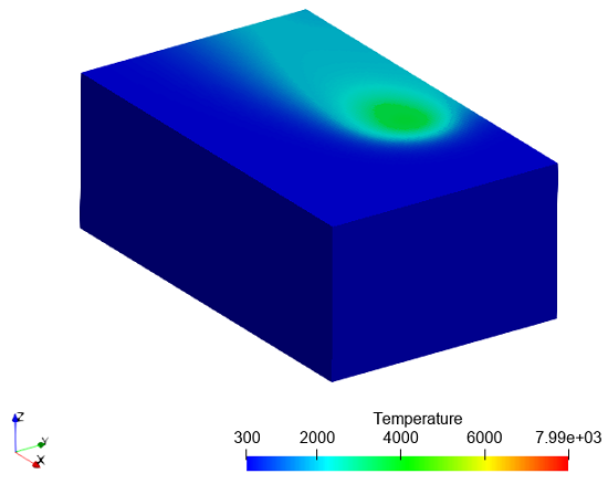
2. Display the temperature distribution field. From the first drop-down list, select Temperature.
Geometry creating, meshing, setting boundary conditions and materials can be performed using the console interface. Below is a link to the program code that allows you to perform the steps described above manual, you only need to specify the full path and name.