Search the documentation
Enter at least 2 characters
Enter at least 2 characters
 |
CAE Fidesys 9.0 Documentation |
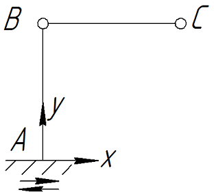
The problem of the dynamic response of the structure under the influence of an earthquake is solved El Centro, defined as a relative displacement response spectrum at a given level of relative damping ζ = 2%. Geometric the problem model is shown in the figure.
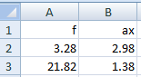
To carry out spectral analysis, you need to prepare a file in the format *.csv with response spectrum. The file should contain a table where the first column contains frequency values (Hz), the subsequent columns contain displacements (speed, acceleration). Column names must be specified:
This table is created as a CSV file and then imported into FidesysViewer (the image shows an example of setting a table in Excel).
Note: Microsoft Excel can open a csv file like this:

i.e. without splitting the file into pillars and listing the values of the lines of the file through comma.
To split text in rows into corresponding columns, you need to list separator settings of your operating system add a comma.
It is worth noting that if the settings are not changed, the file will not download correctly.
1. Create the first straight line.
On the command bar, select the module for constructing geometry (Mode - Geometry, Entity - Curve, Action — Create).
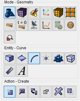
From the list of geometric primitives, select Line. Build using Location and Direction.
Set the parameters:
Location: 0 0 0 (the beginning of the line);
Direction: 0 1 0;
Length: 2.
Click Apply.
2. Create a second straight line.
On the command bar, select the module for constructing geometry (Mode - Geometry, Entity - Curve, Action — Create).
From the list of geometric primitives, select Line. Build using Location and Direction.
Set the parameters:
Location: 0 2 0 (the beginning of the line);
Direction: 1 0 0;
Length: 2.
Click Apply.
As a result, two free curves appeared in the object tree on the left, which have no common vertices.
3. Merge the two vertices.
On the command bar, select the module for constructing geometry (Mode - Geometry, Entity - Vertex, Action - Merge).
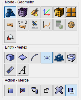
Set parameters:
Vertex ID: 2 3 (separated by a space).
Click Apply.
Enter at the command line: merge all.
1. On the command bar, select the mesh module (Mode - Mesh, Entity - Curve, Action - Mesh).
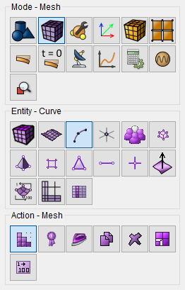
Specify the degree of grinding of the mesh:
Select Curves: all;
Choose the way to build the mesh: Equal;
Select the construction parameters: Interval;
Interval: 10.
Click Apply Size.
Click Mesh.
1. Create the material.
In the command bar, select the module for specifying material properties (Mode - Material, Entity - Materials Management).

In the Materials Management window that opens, in the second column, click with the mouse on the label, specify the name of the material and write "mat1". Click the ENTER.
In the left column, select Elasticity - Isotropic Material. Select the Young's Module characteristic with the mouse. Hold down the left mouse button and drag the label in the properties of the material. Double click in the Value field opposite the Module Young and specify the number 2e+11.
Similarly, from the Isotropic Material section, we add a Poisson ratio of 0.33.
From the General section, we add Density 1e-07.
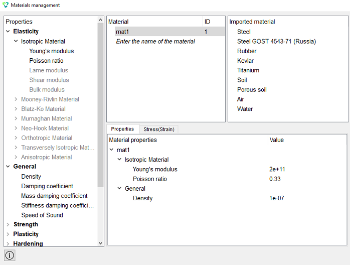
Click Apply.
Close the Materials management window.
2. Create the first block of the same type of material.
On the command bar, select the block management module (Mode - Blocks, Entity - Block, Action — Add).

Set the following parameters:
Block ID: 1;
Entity List: Curve;
Entity ID(s): 1 2 (or all).
Click Apply.
3. Set the block parameters.
On the command bar, select the block management module (Mode - Blocks, Entity - Block, Action — Block properties/parameters).

Set the following parameters:
Block ID(s): 1;
Category: Beam;
Material: Mat 1;
Coordinate System: Global Cartesian;
Order: 1.
Set the properties of the beam, to do this, click on the button  . From the Section profile drop-down list, select Set
parameters manually.
. From the Section profile drop-down list, select Set
parameters manually.
Set the following parameters:
CS Rotation Angle: 0;
Offset to: Centroid;
Use wraping dof;
Y Eccentricity: 0;
Z Eccentricity: 0;
Inertia moment Iy: 4e-07;
Inertia moment Iz: 4e-07;
Inertia moment Ip: 0;
Inertia moment Iyz: 0;
Inertia moment on torison It: 0;
Area: 0.002242;
Max Y coordinate: 0;
Max Z coordinate: 0;
Shear coefficient YY: 1;
Shear coefficient ZZ: 1;
Shear coefficient ZY: 0;
Shear center Y: 0;
Shear center Z: 0;
Wraping constant Iω: 0.
Click Apply.
Close the Set beam properties window.
Click Apply.
4. Create a second block.
On the command bar, select the block management module (Mode - Blocks, Entity - Block, Action — Add).
Set the following parameters:
Block ID: 2;
Entity List: Vertex;
Entity ID(s): 2.
Click Apply.
5. Set the block parameters.
On the command bar, select the block management module (Mode - Blocks, Entity - Block, Action — Block properties/parameters).
Set the following parameters:
Block ID(s): 2;
Category: Lumped Mass;
Coordinate System: Global Cartesian.
Set the properties of the lumped mass, to do this, click on the button
.
Set the following parameters:
Mass: 100;
Inertia Moment: 0.
Click Apply.
Close the Set Lumped Mass Properties window.
Click Apply.
6. Create a third block.
On the command bar, select the block management module (Mode - Blocks, Entity - Block, Action — Add).
Set the following parameters:
Block ID: 3;
Entity List: Vertex;
Entity ID(s): 4.
Click Apply.
7. Set the block parameters.
On the command bar, select the block management module (Mode - Blocks, Entity - Block, Action — Block properties/parameters).
Set the following parameters:
Block ID(s): 3;
Category: Lumped Mass;
Coordinate System: Global Cartesian;
Set the properties of the lumped mass, to do this, click on the button
.
Set the following parameters:
Mass: 200;
Inertia Moment: 0.
Click Apply.
Close the Set Lumped Mass Properties window.
Click Apply.
1. Fix point A in all directions.
On the command panel, select the boundary conditions module (Mode - Boundary Conditions, Entity - Displacement, Action — Create).
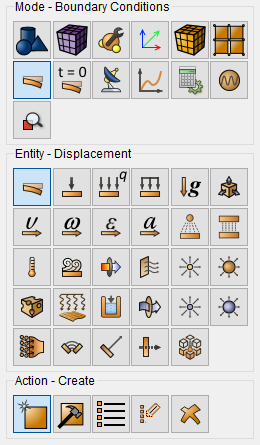
Set the following parameters:
Entity List: Node;
Entity ID(s): 1;
Degrees of Freedom: Fix All.
Click Apply.
2. Fix the model by Z.
On the command panel, select the boundary conditions module (Mode - Boundary Conditions, Entity - Displacement, Action — Create).
Set the following parameters:
Entity List: Curve;
Entity ID(s): all;
Degrees of Freedom: Z.
Click Apply.
1. Specify the type of task you want to solve.
On the command bar, select the calculation settings module (Mode - Calculation Settings, Calculation Settings — Spectrum Analysis, Spectrum analysis - General).
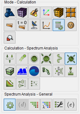
Select:
Dimensions: 3D;
Type: Responce Spectrum;
Number of Eigenmodes: 2.
Click Apply.
Click Start Calculation.
2. In the window that appears, select the directory where the result will be saved and enter the file name.
3. In the case of a successful calculation, the console displays the message: Calculation finished successfully at "date" "time".
1. Open the file with the results. There are three ways to do that.
Click Ctrl+E.
From the main menu, select Calculation. Click Open Results.
Select Results on Command Panel (Mode - Results). Click Open results.

2. Set the response spectrum.
In the main menu, go to the Filters - Alphabetical - Response spectrum.
In the Properties tab, set the following parameters:
Set the flag Absolute Sum;
Set the flag Square Root Of Sum Of Squares;
Set the flag Complete Quadratic Combination;
Constant Mode Damping Ratio: 0.02;
Specify the path of the csv file on your computer;
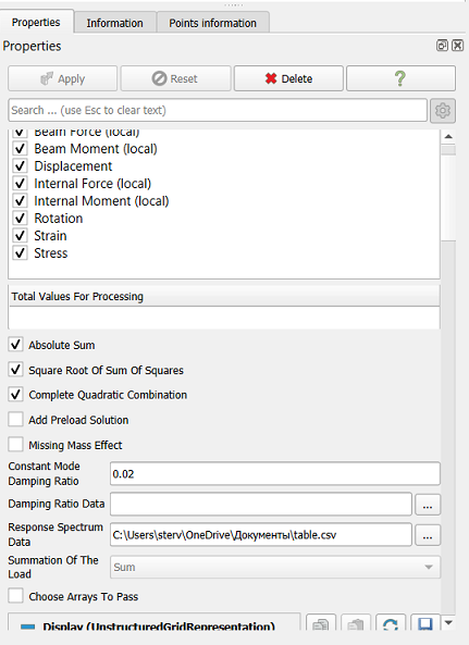
Click Apply.
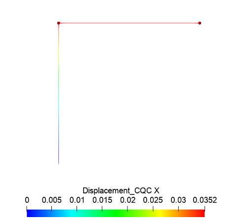
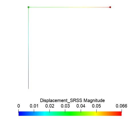
3. Output the results of movements along the X axis obtained by different methods combinations of mods.
In the results drop-down list, select results Displacement_CQC;
In the drop-down list of coordinate axes, select X.

In the results drop-down list, select results Displacement_SRSS;
In the drop-down list of coordinate axes, select Magnitude.

Geometry creating, meshing, setting boundary conditions and materials can be performed using the console interface. Below is a link to the program code that allows you to perform the steps described above manual, you only need to specify the full path and name.