Search the documentation
Enter at least 2 characters
Enter at least 2 characters
 |
CAE Fidesys 9.0 Documentation |
The example describes the calculation of a cylindrical radiator under the action of an internal heat flow. To solve a single-connected thermomechanical problem, the material parameters, including the hardening curve, are specified as temperature-dependent.
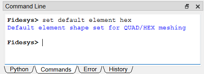
1. Specify a predominantly hexahedral mesh. To do this, enter in the command line: set default element hex .
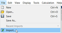
2. Import the geometry.
In the standard line, select Menu — File — Import. Specify the path to the file 05_import_sat.sat. If you cannot download the model, right-click on its name and select Save target as.... Then specify the folder where you want to go. place it.
The file can also be found in the folder C:\Program Files\Fidesys\CAE-Fidesys-9.0\preprocessor\bin\help\fidesys_example_tutorials\TestsFromHelp\models and select the specified model.
In the window that appears, click Finish, leaving all the default parameters.
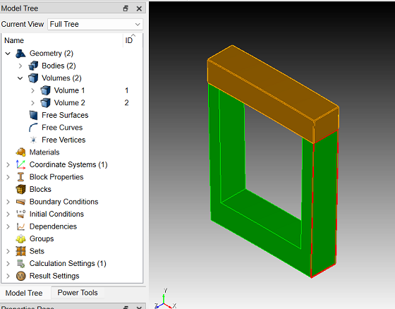
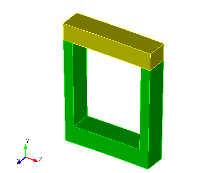
In the Tree on the left you can see two volumes into which the model is divided. All two volumes have no common surfaces.
3. Imprint and merge volumes.
On the command bar, select the module for constructing volume geometry (Mode — Geometry, Entity — Volume, Action — Imprint and Merge).
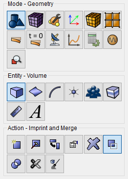
In the pop-up window, select Imprint/Merge Volumes.
Volume ID(s): all.
Click Apply.
1. On the command bar, select the surface mesh construction module (Mode — Mesh, Entity — Surface, Action — Intervals).
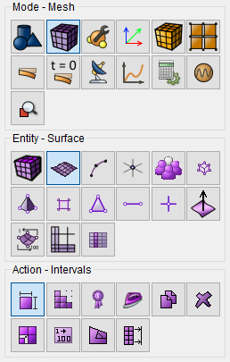
Specify the following parameters:
In the drop-down list, select: Automatic Sizing;
Select Surfaces: 18 2;
Auto Factor: 3.
Click Apply Size.
Click Mesh.
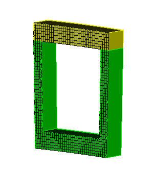
2. On the command bar, select the module for constructing a mesh on curves (Mode — Mesh, Entity — Curve, Action — Mesh).
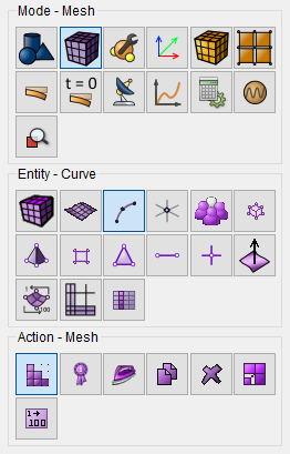
Specify the following parameters:
Select Curves: 48 27 26;
In the drop-down list, select: Equal;
Interval;
Interval: 1.
Click Apply.
3. On the command bar, select the module for constructing a volumetric mesh (Mode — Mesh, Entity— Volume, Action — Intervals).
Specify the following parameters:
In the drop-down list, select: Automatic Sizing;
Select Volumes: 1 2;
Auto Factor: leave default.
Click Mesh.
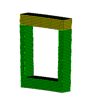
Thus, a conformal finite element mesh was constructed on the model.
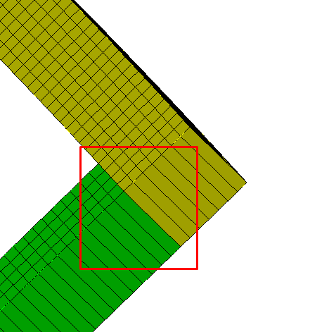
1. Download tables (05_E1.csv, 05_E2.csv, 05_c1.csv, 05_c2.csv, 05_beta1.csv, 05_beta2.csv, 05_sigmay1.csv, 05_hardening2.csv, 05_kappa2.csv, 05_pressure2.csv, 05_pressure1.csv ). To do this, enter the path in the address bar of the explorer: C:\Program Files\Fidesys\CAE-Fidesys-9.0\preprocessor\bin\help\fidesys_example_tutorials\TestsFromHelp\models\Tables and select the specified tables.
2. Specify the material 1.
In the command bar, select the module for specifying material properties (Mode — Material, Entity — Materials Management).

In the opened Material Management widget, in the middle column, specify the name of the material mat_1.
In the properties column, open the Elasticity - Isotropic Material list and drag Young's modulus and Poisson ratio to the Material Properties column.
Next, in the properties column, open the General list and drag Density to the Material Properties column.
Next, in the properties column, open the Plasticity - Mises Criterion list and drag Yield strength to the Material Properties column.
Next, in the properties column, open the Thermal Properties list and drag Thermal Isotropic and Specific heat coefficient to the Material Properties column.
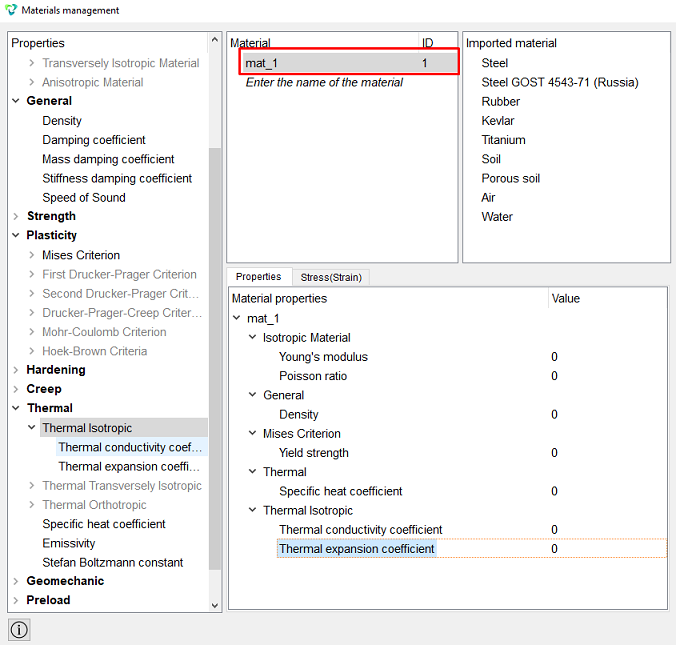
Fill in the properties as follows:
Poisson ratio: 0.3;
Density: 8.9e-09;
Thermal conductivity coefficient: 640.
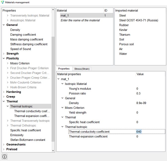
3. Create material 2.
In the Material Management widget, in the middle column, specify the name of the material mat_2.
In the properties column, open the Elasticity - Isotropic Material list and drag Young's modulus and Poisson ratio to the Material Properties column.
Next, in the properties column, open the General list and drag Density to the Material Properties column.
Next, in the properties column, open the Plasticity - Mises Criterion list and drag Yield strength to the Material Properties column.
Next, in the properties column, open the Hardening - Polylinear Isotropic list and drag Stress(Strain) curve to the Material Properties column.
Next, in the properties column, open the Thermal Properties list and drag Temperature Isotropic and Specific heat coefficient to the Material Properties column.
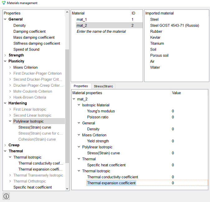
Fill in the properties as follows:
Poisson ratio: 0.3;
Density: 7.8e-09;
Yield strength: 665.
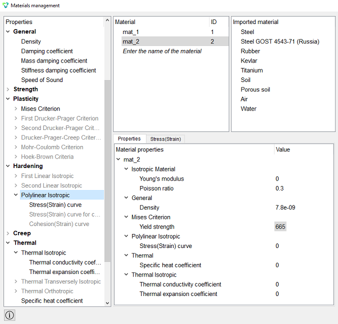
4. Import tables for material 1.
Click on 0 next to Young's modulus and click on ... to add a table.
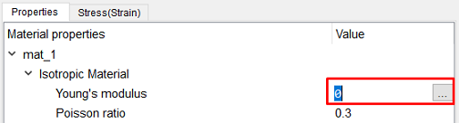
Next, click Import and import the saved table 05_E1.csv.
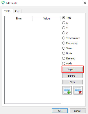
Click on the temperature to add the required column.
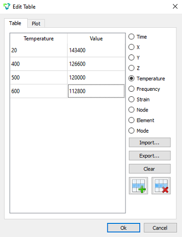
Click Ok.
Click on 0 next to Specific heat coefficient and click on ... to add the table.
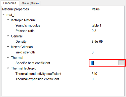
Click Import and import the saved table 05_c1.csv.
Click on the temperature to add the required column.
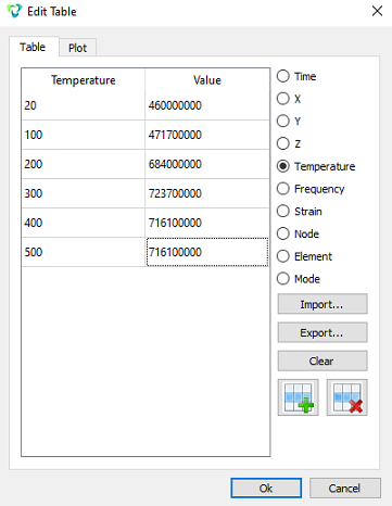
Click Ok.
Click on 0 next to Thermal expansion coefficient of and click on ... to add the table.
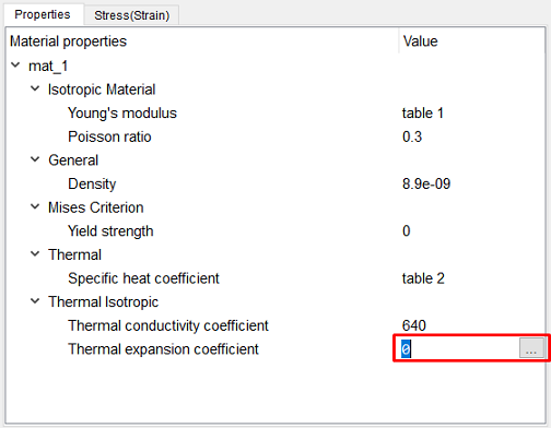
Click Import and import the saved 05_beta1.csv table.
Click on the temperature to add the required column.
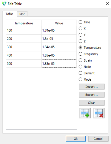
Click Ok.
Click on 0 next to Yield strength and click on ... to add the table.
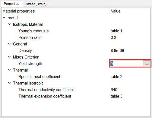
Click Import and import the saved table 05_sigmay1.csv.
Click on the temperature to add the required column.
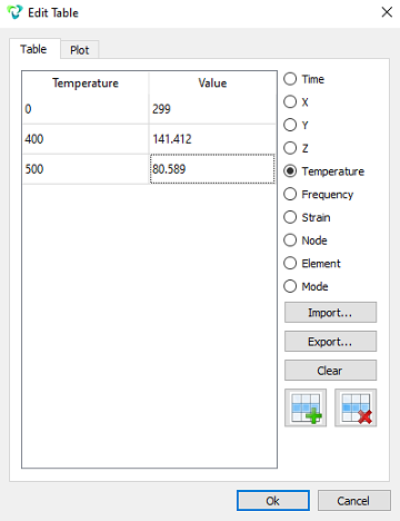
Click Ok.
Click Apply.
Close the Material Management window.
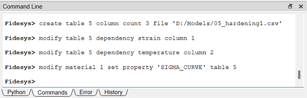
5. Import the table for the Material Stress/Strain Curve parameter 1.
Enter the following in the command line:
Note: Don't forget to change the path in the command!
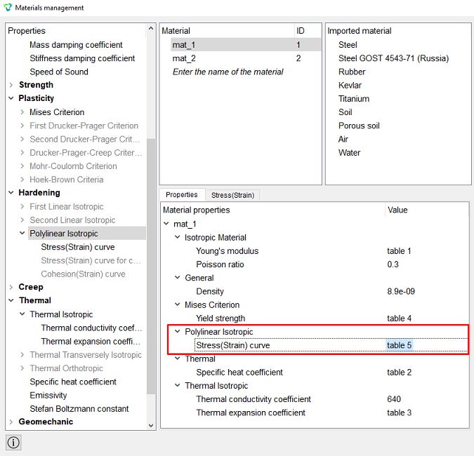
On the command bar, select the module for setting material properties (Mode — Material, Entity— Material Management).
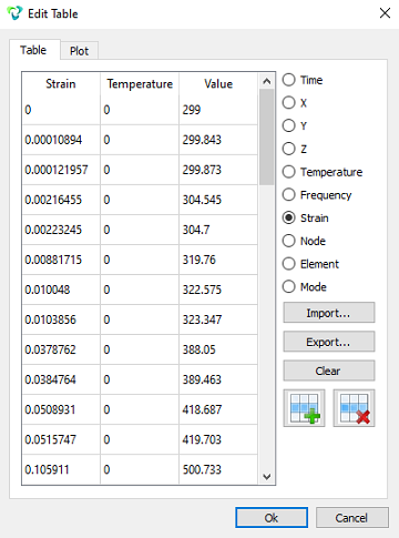
In the widget that opens, click on mat_1. And check table 5 in the parameter Stress(Strain) curve.
5. Fill in the tables for material 2.
Click on 0 next to Young's modulus and click on ... to add a table. Next, click Import and import the saved table 05_E2.csv.
Click on temperature to add the required column.
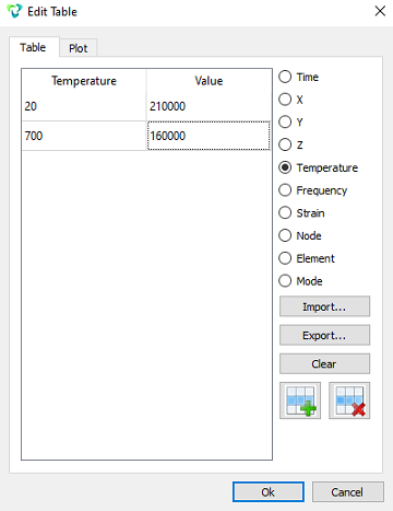
Click Ok.
Click on 0 next to Specific heat coefficient and click on ... to add the table. Click Import and import the saved table 05_c2.csv.
Click on temperature to add the required column.
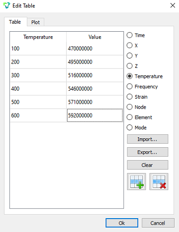
Click Ok.
Click on 0 next to Thermal conductivity coefficient and click on ... to add the table. Click Import and import the saved table 05_kappa2.csv.
Click on temperature to add the required column.
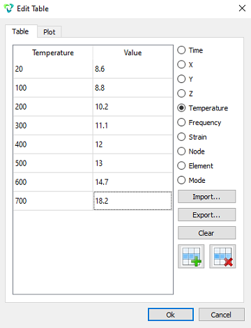
Click Ok.
Click on 0 next to Thermal expansion coefficient and click on ... to add the table. Click Import and import the saved table 05_beta2.csv.
Click on temperature to add the required column.
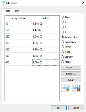
Click Ok.
Click on 0 next to Stress(Strain) curve and click on ... to add the table. Click Import and import the saved table 05_hardening2.csv.
Click on plastic strain to add the required column.
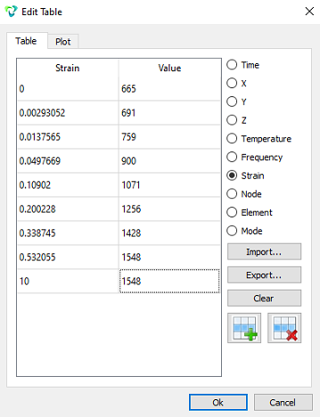
Click Ok.
Click Apply.
Close the Material Management window.
6. Create the first block.
On the command bar, select the block management module (Mode — Blocks, Entity — Block, Action — Add).

Specify the following parameters:
Block ID: 1;
Entity List: Volume;
Entity ID(s): 1.
Click Apply.
7. Set the block parameters.
On the command bar, select the block management module (Mode — Blocks, Entity— Block, Action — Block properties/parameters).

Set the following parameters:
Block ID(s): 1;
Category: Solid;
Material: mat_1;
Coordinate System: Global Cartesian;
Order: 2.
Click Apply.
8. Create the second block.
On the command bar, select the block management module (Mode — Blocks, Entity — Block, Action — Add).
Specify the following parameters:
Block ID: 2;
Entity List: Volume;
Entity ID(s): 2.
Click Apply.
9. Set the block parameters.
On the command bar, select the block management module (Mode — Blocks, Entity — Block, Action — Block properties/parameters).
Set the following parameters:
Block ID(s): 2;
Category: Solid;
Material: mat_2;
Coordinate System: Global Cartesian;
Order: 2.
Click Apply.
1. Fix the sides of the volumes.
On the command bar, select the boundary conditions module (Mode — Boundary Conditions, Entity — Displacement, Action — Create).
Set the following parameters:
Entity List: Surface;
Entity ID(s): 2 4 11 18 (or select surfaces with the mouse while holding down the Ctrl key);
Degrees of Freedom: Z-Translation Disp;
DOF Value: 0 (can be left blank).
Click Apply.
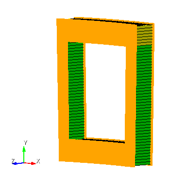
2. Fix the sides of the model in a direction.
On the command bar, select the boundary conditions module (Mode — Boundary Conditions, Entity — Direction Restraint, Action — Create).
Set the following parameters:
Entity List: Surface;
Entity ID(s): 15 6 8 17 (or select surfaces with the mouse while holding down the Ctrl key);
Type: Displacement;
Direction: Normal;
Value: 0.
Click Apply.
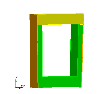
3. Set the initial temperature.
On the command bar, select the module for setting initial conditions (Mode — Initial Conditions, Entity — Temperature, Action — Create).
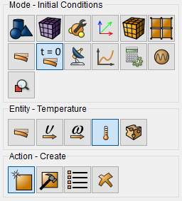
Set the following parameters:
Entity List: Volume;
Entity ID(s): all;
Value: 360.9.
Click Apply.
4. Set convection to the interior of the model.
On the command bar, select the boundary conditions module (Mode — Boundary Conditions, Entity — Convection, Action — Create).
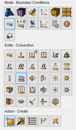
Set the following parameters:
Entity List: Surface;
Entity ID(s): 3 1 13 10;
Surrounding;
Temperature: 360.9;
Coefficient: 28.9.
Click Apply.
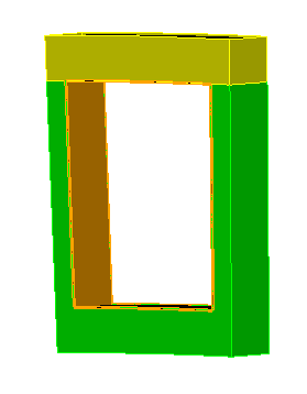
5. Set the heat flux.
On the command bar, select the boundary conditions module (Mode — Boundary Conditions, Entity — Heatflux, Action — Create).
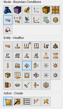
Set the following parameters:
Entity List: Surface;
Entity ID(s): 7;
Surrounding;
Flux: 13685.
Click Apply.
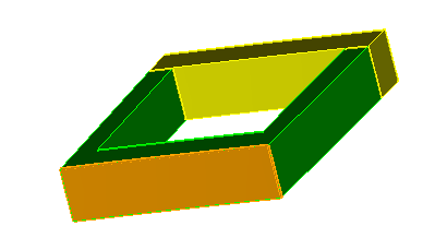
6. Set the pressure on the interior of the model.
On the command bar, select the boundary conditions module (Mode — Boundary Conditions, Entity — Pressure, Action — Create).
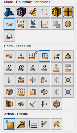
Set the following parameters:
Pressure Entity List: Surface;
Entity ID(s): 3 1 13 10;
Magnitude Value: 1.
Click Apply.
7. Set the pressure on the bottom of the model.
On the command bar, select the boundary conditions module (Mode — Boundary Conditions, Entity — Pressure, Action — Create).
Set the following parameters:
Pressure Entity List: Surface;
Entity ID(s): 7;
Magnitude Value: 2.
Click Apply.
8. Import the table for pressure 2.
On the command bar, select the boundary conditions module (Mode — BC Dependency).
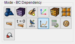
For Pressure 2, do:
Click on the "Table" tab and click Import. Import the saved table 05_pressure2.csv.
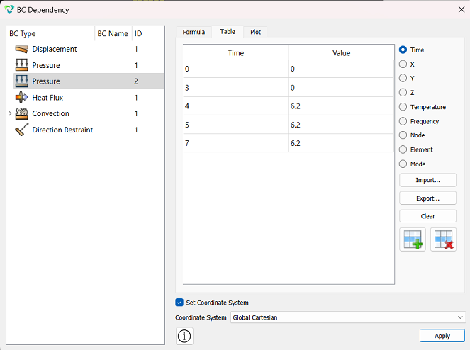
Click Apply.
9. Import the table for pressure 1.
For Pressure 1, do the following:
Click the "Table" tab and click Import. Import the saved table 05_pressure1.csv.
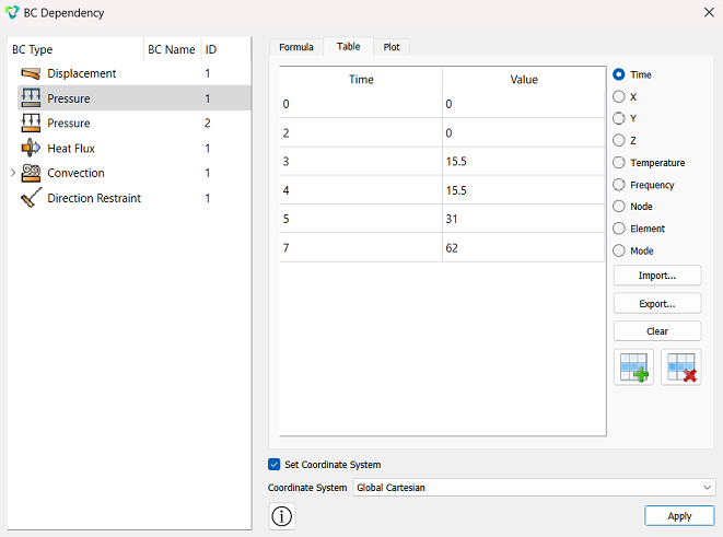
Click Apply.
Close the BC Dependency window.
1. Specify the type of problem to be solved.
On the command bar, select the calculation settings module (Mode — Calculation Settings, Calculation Settings —Transient Analysis, Transient — General).
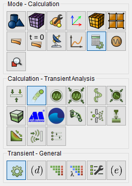
Set the following calculation parameters:
Dimensions: 3D;
Method: Full solution;
Scheme: Implicit;
Max time: 4;
Time step: 0.12;
Elasticity:
Plasticity;
Nonlinear geometry.
Heat transfer;
Set nonlinear solver options:
Start load substeps: 10;
Min load substeps: 1;
Max load substeps: 100000000;
Max iterations: 1000;
Tolerance: 1e-6;
Target iterations: 4.
Set implicit scheme options;
Newmark algoritm gamma: 0.4.
Click Apply.
2. Set additional task parameters.
On the command bar, select the calculation settings module (Mode — Calculation Settings, Calculation Settings —TransientAnalysis, Transient — Environment Properties).
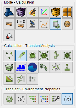
Temperature: 366.9
Click Apply.
Click Start Calculation.
3. In a pop-up window select a folder to save the result and enter the file name.
4. In the case of a successful calculation, the console displays the message: Calculation finished successfully at "date" "time".
1. Open the file with the results. There are three ways to do that.
Click Ctrl+E.
From the main menu, select Calculation. Click Open Results.
Select Results on Command Panel (Mode - Results). Click Open results.

The FidesysViewer window will appear, where you can view the calculation results.
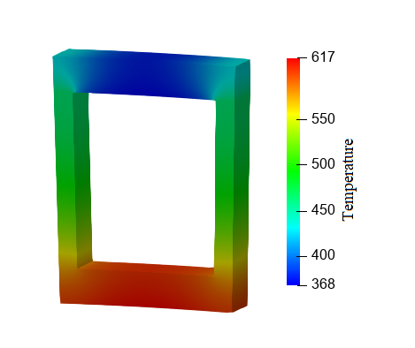
2. Display the temperature values for the model.
From the first drop-down list, select Temperature.
3. Display the plastic strain values for the model.
From the first drop-down list, select Elastic Strain, from the second – Mises.
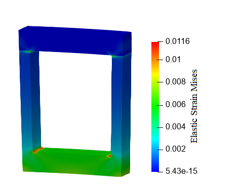
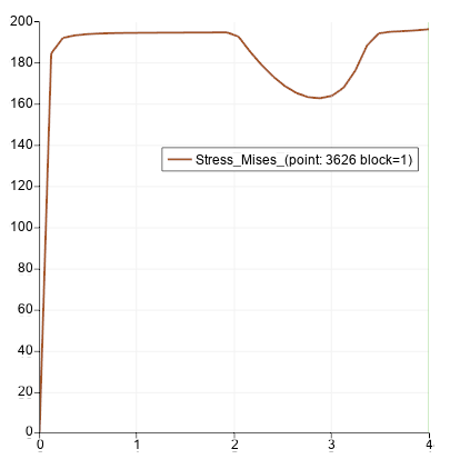
3. Display a graph of stress versus time.
From the first drop-down list, select Stress, from the second – Mises. Select the display Surface With Edges.
On the main panel of FidesysViewer, click Select Points On surface. Select a point on the model.
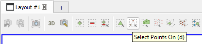
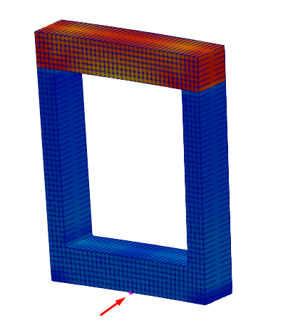
On the command bar, select Filters — Alphabetical — Plot Selection Over Time.
In the properties, click Apply. Then in the properties, select display von Mises stresses.
Geometry creating, meshing, setting boundary conditions and materials can be performed using the console interface. Below is a link to the program code that allows you to perform the steps described above manual, you only need to specify the full path and name.