Search the documentation
Enter at least 2 characters
Enter at least 2 characters
 |
CAE Fidesys 9.0 Documentation |
Stress-strain state in the vicinity of a vertical well of radius Rw drilled to a depth of h is determined. The reservoir is considered to be isotropic and homogeneous. The problem is solved in a cylindrical coordinate system.
1. Create the first circle with radius 10.
On the command bar, select the module for constructing surface geometry (Mode — Geometry, Entity— Surface, Action — Create).
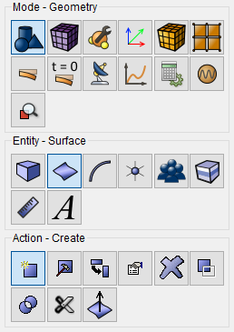
Select Circle in the list of geometric elements.
Set block sizes:
Radius: 10;
Location: ZPlane.
Click Apply.
2. Create the second circle with radius 1.
On the command bar, select the module for constructing surface geometry (Mode - Geometry, Entity - Surface, Action - Create).
From the list of geometric primitives, select Circle.
Set block sizes:
Radius: 1;
Location: ZPlane.
Click Apply.
3. Subtract the first circle from the second one.
On the command bar, select the module for constructing surface geometry (Mode — Geometry, Entity — Surface, Action — Boolean).
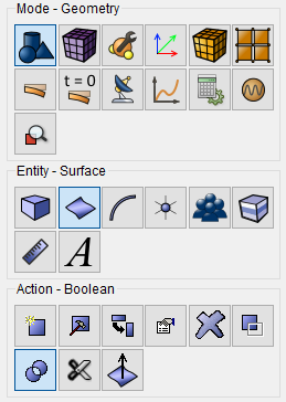
Select Subtract in the list of operations.
Set the following parameters:
A Surface ID(s): 1;
B Surface ID(s: 2.
Click Apply.
As a result, only one body (Body 1) will remain in the model tree.
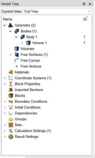
4. Leave a quarter of the volume (condition of symmetry).
On the command bar, select the module for constructing surface geometry (Mode — Geometry, Entity — Surface, Action — Webcut).
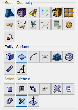
From the list of available section views select Coordinate Plane.
Set the following parameters:
Body ID(s): 1;
Cut Plane: ZX;
Offset Value: 0.
Click Apply.
Do the same, but in the YZ plane:
Body ID(s): 3;
Cut Plane: YZ;
Offset Value: 0.
Click Apply.
Then delete volumes 4 and 1.

5. On the command bar, select the module for constructing volume geometry (Mode — Geometry, Entity — Volume, Action — Delete).
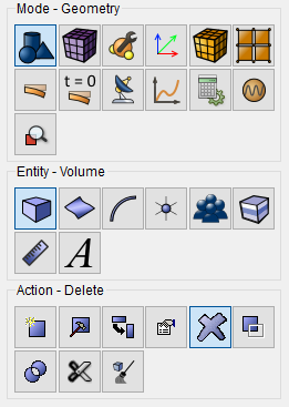
Set the following parameters:
Volume ID(s): 4 1 (separated by a space).
Click Apply.
1. In the command bar, select the module for specifying material properties (Mode — Material, Entity — Material Management).

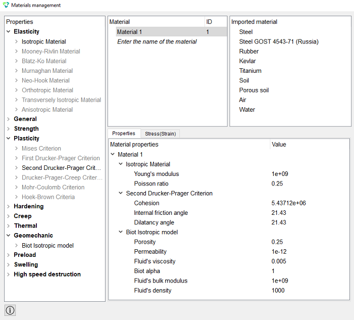
Specify the name of the material Material 1. Expand the item Elasticity in the left column and drag the Isotropic Material to the Material Properties column. Set the following parameters:
Young's modulus: 1e+9;
Poisson ratio: 0.25.
Expand Plasticity in the left column and drag the Second Drucker-Prager Strength Criterion into the Material Properties column. Set the following parameters:
Cohesion: 5.43712e+06;
Internal friction angle: 21.43;
Dilatancy angle: 21.43.
Expand Geomechanics in the left column and drag Bio Isotropic Model to the Material Properties column. Set the following parameters:
Porosity: 0.25;
Permeability: 1e-12;
Fluid's viscosity : 0.005;
Biot alpha: 1;
Fluid's bulk modulus: 1e+09;
Fluid's density: 1000.
Click Apply.
Close the Materials management window.
1. On the command bar, select the mesh module (Mode — Mesh, Entity — Curve, Action — Mesh).
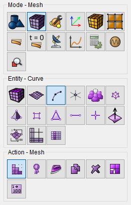
Specify the parameters of mesh refinement:
Select Curves: 8;
Bias;
Intervals and Bias;
Change Interval Count;
Interval Count: 90;
Bias Factor: 1.05;
Start Vertex ID: 7.
Click Apply.
2. On the command bar, select the mesh module (Mode — Mesh, Entity — Curve, Action — Mesh).
Specify the parameters of mesh refinement:
Select Curves: 12;
Bias;
Intervals and Bias;
Change Interval Count;
Interval Count: 90;
Bias Factor: 1.05;
Start Vertex ID: 11.
Click Apply.
3. On the command bar, select the mesh module (Mode — Mesh, Entity — Curve, Action — Mesh).
Specify the parameters of mesh refinement:
Select Curves: 13 14 (separated by a space);
Equal;
Interval;
Interval: 30.
Click Apply.
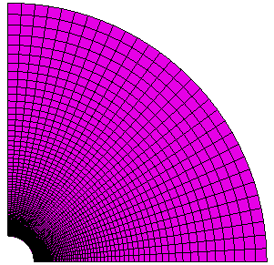
4. Building the mesh.
On the command bar, select the surface mesh module (Mode — Mesh, Entity — Surface, Action — Mesh).
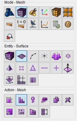
Specify the degree of mesh refinement:
Automatically Calculate;
Select Surfaces: all.
Click Mesh.
1. Attach curves 8 and 12 in the direction Y and X respectively.
On the command panel, select the boundary conditions module (Mode - Boundary Conditions, Entity - Displacement, Action - Create).
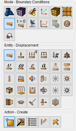
Set the following parameters:
Entity List: Curve;
Entity ID(s): 8;
Degrees of Freedom: Y.
Click Apply.
Set the following parameters:
Entity List: Curve;
Entity ID(s): 12;
Degrees of Freedom: X.
Click Apply.
2. Set the pore pressure.
On the command panel, select the boundary conditions module (Mode - Boundary Conditions, Entity – Pore Pressure, Action - Create).
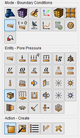
Set the following parameters:
Entity List: Curve;
Entity ID(s): 13 14 (separated by a space);
Value: 4e+7.
Click Apply.
3. Set the pressure on curves 13 and 14.
On the command panel, select the boundary conditions module (Mode - Boundary Conditions, Entity – Pressure, Action - Create).
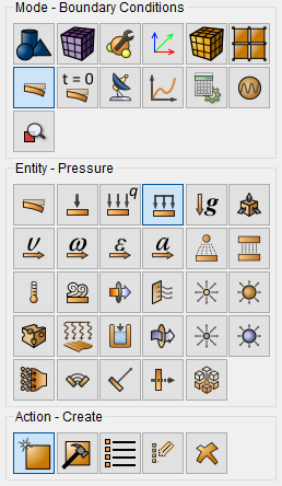
Set the following parameters:
Entity List: Curve;
Entity ID(s): 13;
Value: 4e+7.
Click Apply.
Set the following parameters:
Entity List: Curve;
Entity ID(s): 14;
Value: 8e+7.
Click Apply.
1. Create a block of one material type.
On the command bar, select the block management module (Mode — Blocks, Entity — Block, Action — Add).

Set the following parameters:
Block ID: 1;
Entity List: Surface;
Entity ID(s): All.
Click Apply.
2. Set the block parameters.
On the command bar, select the block management module (Mode - Blocks, Entity - Block, Action - Block properties/parameters).

Set the following parameters:
Block ID(s): 1;
Category: Plane;
Material: Material 1;
Coordinate System: Global Cartesian;
Order: 2.
Click Apply .
1. Set the analysis type.
On the command bar, select the calculation settings module (Mode — Calculation Settings, Calculation Settings — Static, Static — General).
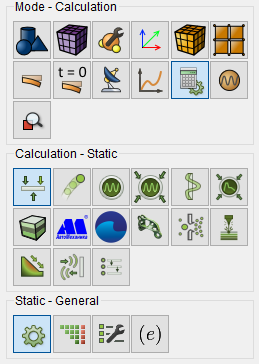
Select:
Dimension: 2D;
Plane State: Plane Strain;
Model: Elasticity, Plasticity, Pore Fluid Transfer;
Set Nonlinear Solver Options;
Min Load Substeps: 30;
Max Load Substeps: 10000000;
Max Iterations: 100;
Tolerance: 1e-6;
Target Iterations: 5.
Click Apply.
Click Start Calculation.
2. In the window that appears, select the directory in which the result will be saved, and enter the file name.
3. In the case of a successful calculation, the console displays the message: Calculation finished successfully at "date" "time".
1. Open the file with the results. There are three ways to do that.
Click Ctrl+E.
From the main menu, select Calculation. Click Open Results.
Select Results on Command Panel (Mode - Results). Click Open results.

The FidesysViewer window will appear, in which you can view the calculation results.
2. On the toolbar, select Filters → Alphabetical → Coordinate System Conversions.
In the Properties window that opens, set:
Coordinate System: Create New;
Type: Cylindrical;
Set By: Directional Vectors.
Coordinate system parameters: Center: 0; 0; 0;
Coordinate system parameters: Z Axis: 0; 0; 1;
Point Values For Processing: Stress.
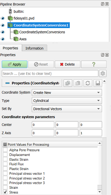
Click Apply.
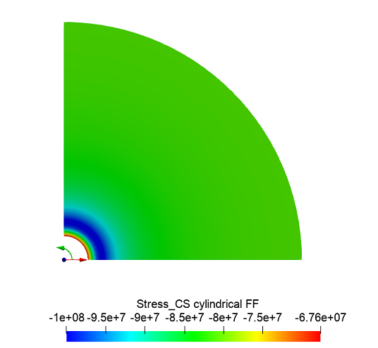
3. Display the σθθ component of the stress field (cylinder) on the model.
On the toolbar, set the following parameters:
Display type: Surface;
Display field: Stress_CS cylindrical;
Display component: FF.

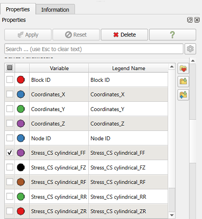
4. On the toolbar, select Filters → Alphabetical → Plot Over Line. In the Properties window that opens, set:
Click Apply;
Row parameters: untick the Variable box;
Row parameters: tick the box Stress_CS cylindrical_FF.
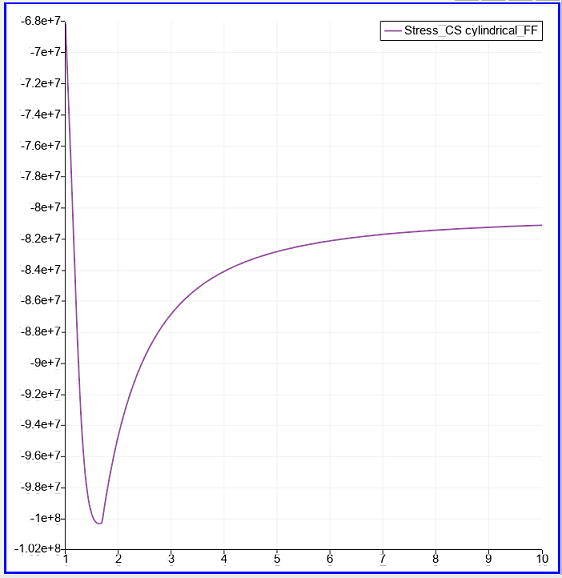
Geometry creating, meshing, setting boundary conditions and materials can be performed using the console interface. Below is a link to the program code that allows you to perform the steps described above manual, you only need to specify the full path and name.