Search the documentation
Enter at least 2 characters
Enter at least 2 characters
 |
CAE Fidesys 9.0 Documentation |
Hinton E. Fundamental Tests for Two and Three-dimensional, Small Strain, Elastoplastic Finite Element Analysis / Emest Hinton, M.H. Ezatt. - NAFEMS, 1987.
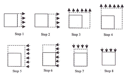
We solve the problem of tension-compression of a square plate. Material parameters: E = 250e3 N / mm2, n = 0.25, yield strength c = 5 N / mm2. The model is meshed into one finite element. The left and bottom sides are fixed perpendicularly. The boundary conditions are presented in the figure below:
1. Create a square plate.
On the command bar, select the module for constructing surface geometry (Mode - Geometry, Entity - Surface, Action - Create).
From the list of geometric primitives, select Rectangle.
Set block sizes:
Width: 1;
Location: ZPlane.
Click Apply.
2. Move the surface to the origin of CS.
On the command bar, select the module for constructing surface geometry (Mode - Geometry, Entity - Surface, Action - Transform).
From the list of possible transformations, select Move.
Set the parameters:
Surface ID(s): 1;
Including Merged: uncheck;
Select Method: Distance;
X Distance: 0.5;
Y Distance: 0.5.
Click Apply.
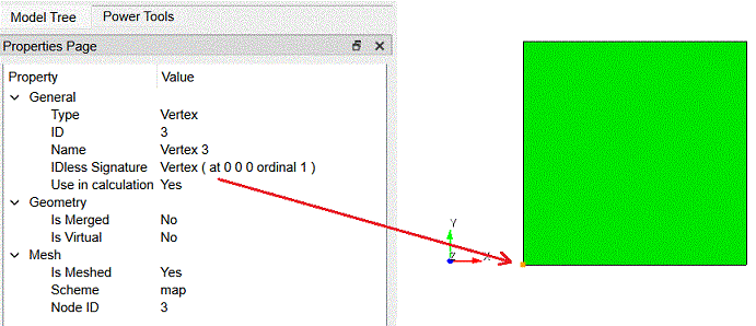
Thus, the lower left corner of the plate has moved to the origin of CS.
1. On the command bar, select the mesh module (Mode - Mesh, Entity - Curve, Action - Mesh).
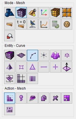
Specify the degree of refining mesh:
Select Curves: all;
Select the meshing method: Equal;
Select the meshing options: Interval;
Interval: 1.
Click Apply Size.
Click Mesh.
2. On the command bar, select the surface mesh module (Mode - Mesh, Entity - Surface, Action - Mesh).
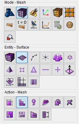
Specify:
Select the mesh scheme: Automatically Calculate;
Select Surfaces: all.
Click Apply Scheme.
Click Mesh.
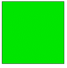
1. Create material.
In the command bar, select the module for specifying material properties
(Mode - Material, Entity - Materials Management).

Specify the name of the material Material 1. Drag the Isotropic Material inscription from the left column into the Material Properties column. Set the following parameters:
Young’s modulus: 250e3;
Poisson ratio: 0.25;
In the window on the left, go to the section Plasticity – Mises Criterion. Drag the Yield strength feature into the Material Properties window. Enter value:
Yield strength: 5.
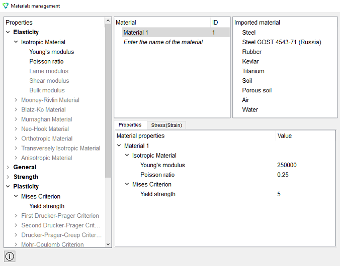
Click Apply.
Close the Materials management window.
2. Create a block of the one type of material.
On the command bar, select the block management module (Mode - Blocks, Entity - Block, Action - Add).

Set the following parameters:
Block ID: 1;
Entity List: Surface;
Entity ID(s): 1 (or by command all).
Click Apply.
3. Set the block parameters.
On the command bar, select the block management module (Mode - Blocks, Entity - Block, Action - Block properties/parameters).

Set the following parameters:
Block ID(s): 1;
Category: Plane;
Material: Material 1;
Coordinate System: Global Cartesian;
Order: 2.
Click Apply.
1. Fix curve 3 in the Y direction.
On the command panel, select the boundary conditions module (Mode - Boundary Conditions, Entity - Displacement, Action - Create).
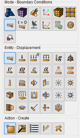
Set the following parameters:
Entity List: Curve;
Entity ID(s): 3;
Degrees of Freedom: Y-Translation Disp;
DOF Value: 0.
Click Apply.
2. Fix curve 2 in the X direction.
On the command panel, select the boundary conditions module (Mode - Boundary Conditions, Entity - Displacement, Action - Create).
Set the following parameters:
Entity List: Curve;
Entity ID(s): 2;
Degrees of Freedom: X-Translation Disp;
DOF Value: 0.
Click Apply.
3. Fix curve 4 in the X direction.
On the command panel, select the boundary conditions module (Mode - Boundary Conditions, Entity - Displacement, Action - Create).
Set the following parameters:
Entity List: Curve;
Entity ID(s): 4;
Degrees of Freedom: X-Translation Disp;
DOF Value: 0.
Click Apply.
4. Fix curve 1 in the Y direction.
On the command panel, select the boundary conditions module (Mode - Boundary Conditions, Entity - Displacement, Action - Create).
Set the following parameters:
Click Apply.
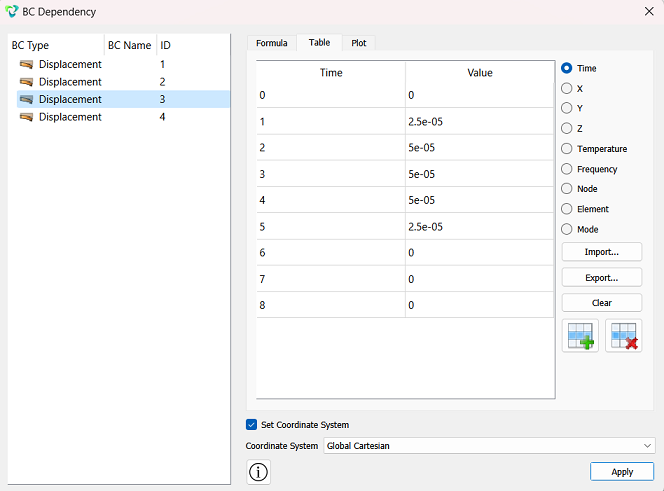
1. Create table 1 for displacement 3.
On the command panel, select the module for specifying Dependency BC (Mode - BC Dependency).
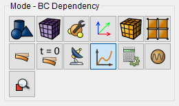
Next, in the left column, click on Displacement 3 and switch to the Table tab. Set the following parameters:
Set the flag: Time;
Add rows by clicking the green plus button 9 times;
Fill the table as follows:
:
Click Apply.
2. Create table 2 for displacement 4.
Click Displacement 4 and choose panel Table in the
right side. Set the flag: Time and fill in the table as follows: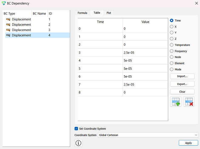
Click Apply.
1. Set the type of problem you want to solve.
On the command bar, select the calculation settings module (Mode - Calculation Settings, Calculation Settings - Static, Static - General).
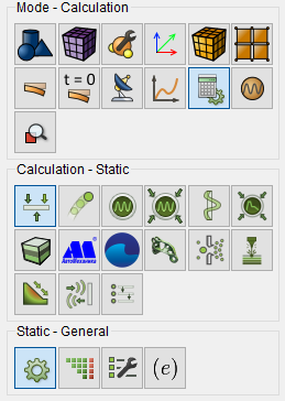
Set the following parameters:
Dimensions: 2D;
Plain state: Plane strain;
Model: Elasticity, Plasticity;
Set static load steps count;
Load steps count: 8.
Click Apply.
Click Start Calculation.
2. In the window that appears, select the directory in which the result will be saved, and enter the file name.
3. In the case of a successful calculation, the console displays the message: Calculation finished successfully at "date" "time".
1. Open the file with the results. There are three ways to do that.
Click Ctrl+E.
From the main menu, select Calculation. Click Open Results.
Select Results on Command Panel (Mode - Results). Click Open results.

To analyze the results, go to the FidesysViewer window.
To automatically apply changes to all filters, click the corresponding
button Apply changes to parameters automatically on the
command bar -  .
.
2. Connect the filter to Warp By Vector (Menu - Filters - Alphabetical - Warp By Vector). Or use the corresponding button on the command bar.

For this filter, on the Properties tab, set:
Vectors: Displacement;
Scale Factor: 10000.
Click Apply (unless Apply changes to parameters automatically is enabled).
3. In the top pane, select the payroll result data to display. From the first drop-down list, select Displacement, from the second - Magnitude.

4. In the step view panel, set step 1. You should see an image of the
plate in its initial state. Next, click Play -  .
You should see the plate sequentially stretching and then compressing
according to the loading history.
.
You should see the plate sequentially stretching and then compressing
according to the loading history.
You should see the plate image in the initial state. Next, click on
Play. You should see a consistent stretching, and then compression of
the plate in accordance with the loading history.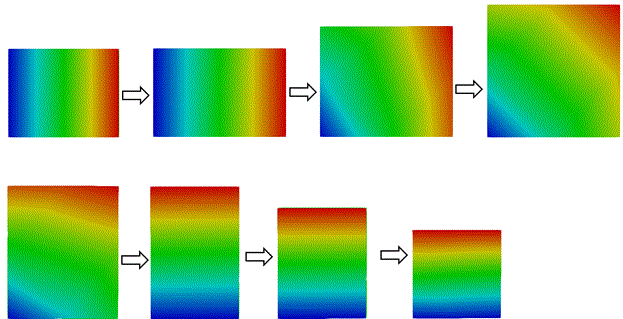
Thus, the calculation of the stress-strain state with the loading history of the plate was made.
Geometry creating, meshing, setting boundary conditions and materials can be performed using the console interface. Below is a link to the program code that allows you to perform the steps described above manual, you only need to specify the full path and name.