Search the documentation
Enter at least 2 characters
Enter at least 2 characters
 |
CAE Fidesys 9.0 Documentation |
The problem of finding the plastic zone around the well in the dynamics, taking into account the pore pressure until instability appears in the form of plastic deformation bands, is solved.
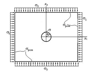
A square plate of considerable width and unit thickness with a small circular hole of radius a in its center is subjected to all-round uniform pressures with stresses σ1 in the direction of the X1 axis and σ2 in the direction of the X2 axis. The lateral faces are affected by time-dependent pore pressure. A round hole is subject to pressure, which is also time dependent.
It is required to calculate plastic zones around the well in dynamics.
1. Create a surface.
On the command bar, select the module for constructing surface geometry (Mode - Geometry, Entity - Surface, Action - Create).
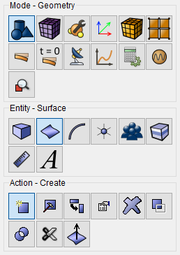
From the list of geometric primitives, select Rectangle.
Set block sizes:
Click Apply.
2. Moving to the origin of the coordinate system.
It is required to move the surface so that one of the vertices is at the origin of the coordinate system.
On the command bar, select the module for constructing surface geometry (Mode - Geometry, Entity - Surface, Action - Transform).
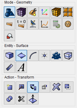
From the list of geometric primitives, select Move.
Set the movement parameters:
Click Apply.
3. Selection of geometric entities
In the standard line we find the panel with the choice of geometric entities.
Click Select Vertices.
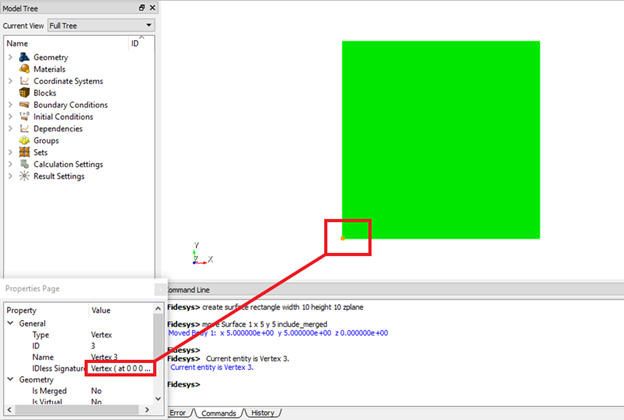
Click on the left bottom vertex of the created surface and look at the obtained coordinates on the Properties Page on the left. Make sure that the vertex has moved to the origin.
4. Creating a circular hole.
It is required to make a cut in the plate using an auxiliary circle.
On the command bar, select the module for constructing surface geometry (Mode - Geometry, Entity - Surface, Action - Create).
From the list of geometric primitives, select Circle.
Set block sizes:
Click Apply.
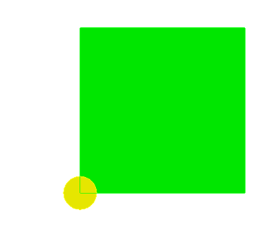
5. On the command bar, select the module for constructing surface geometry (Mode - Geometry, Entity - Surface, Action - Boolean).
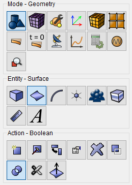
From the list of logical operations, select Subtract.
Set the parameters of the logical operation:
A Surface ID(s): 1;
B Surface ID(s): 2.
Click Apply.

1. Changing the mesh settings.
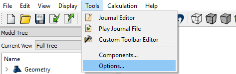
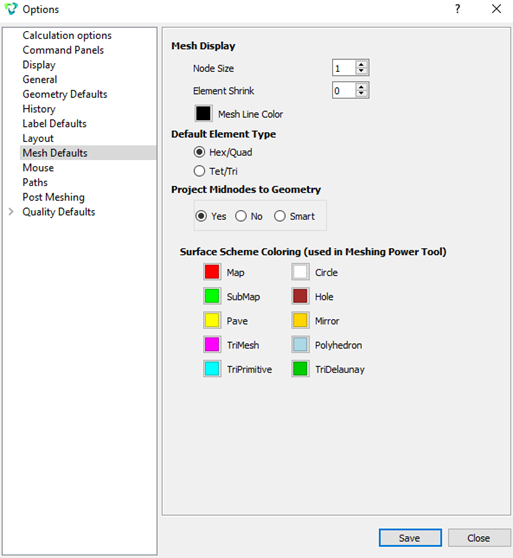
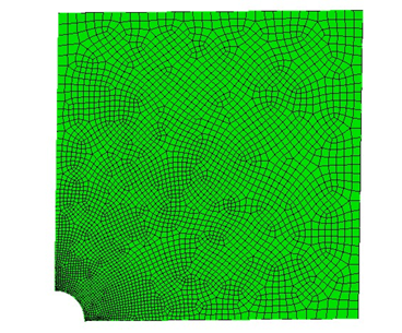
To automatically create a quadrilateral mesh, we will change the default settings. In the standard line, select Tools - Settings. In the opened window in the left column select the Mesh Defaults. On the Default Element Type panel we select the Hex / Quad.
Click Save.
2. On the command bar, select the mesh module (Mode - Mesh, Entity - Curve, Action - Mesh).
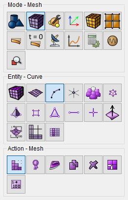
Specify the degree of reducing mesh:
Click Apply Size.
Click Mesh.
3. On the command bar, select the mesh module (Mode - Mesh, Entity - Curve, Action - Mesh).
Specify the degree of reducing mesh:
Click Apply Size.
Click Mesh.
4. On the command bar, select the mesh module (Mode - Mesh, Entity - Curve, Action - Mesh).
Specify the degree of reducing mesh:
Click Apply Size.
Click Mesh.
5. On the command bar, select the surface mesh module (Mode - Mesh, Entity - Surface, Action - Intervals).
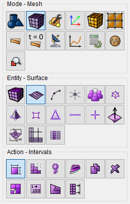
Click Mesh.
1. Create a material.
In the command bar, select the module for specifying material properties (Mode —Material, Entity - Materials Management).

In the Material Management widget that opens, in the middle column specify the name of the material. In the properties column, open the Elasticity list and drag the name Isotropic Material into the Material Properties column.
Set the following parameters:
In the left column, go to the General section and select Density. Drag the mouse into the right column and specify the value 2650.
In the left column, go to the Plasticity section and select the Drucker-Prager Second Strength Criterion.
In the left column go to the section Geomechanics - Biot Isotropic model.
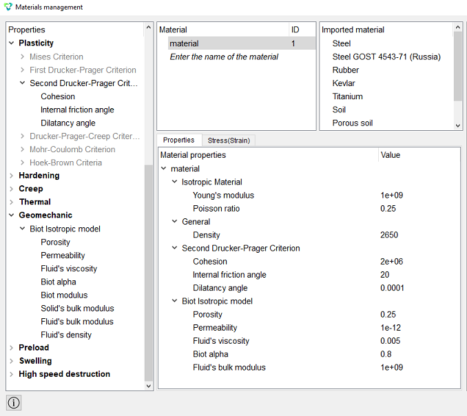
Click Apply.
Close the Materials management window.
2. Create a block of the one type of material.
On the command bar, select the block management module (Mode - Blocks, Entity - Block, Action - Add).

Set the following parameters:
Click Apply.
3. Set the block parameters.
On the command bar, select the block management module (Mode - Blocks, Entity - Block, Action - Block properties/parameters).

Set the following parameters:
Block ID(s): 1;
Category: Plane;
Material: Material1;
Coordinate System: Global Cartesian;
Order: 2.
Click Apply.
1. Apply pressure to the right side curve.
On the command panel, select the boundary conditions module (Mode - Boundary Conditions, Entity - Pressure, Action - Create).
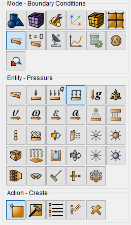
Set the following parameters:
Click Apply.
2. Apply pressure to the right side curve.
On the command panel, select the boundary conditions module (Mode - Boundary Conditions, Entity - Pressure, Action - Create).
Set the following parameters:
Click Apply.
3. Set the time-dependent load on the model's notch.
On the command panel, select the boundary conditions module (Mode - Boundary Conditions, Entity - Pressure, Action - Create).
Set the following parameters:
Click Apply.
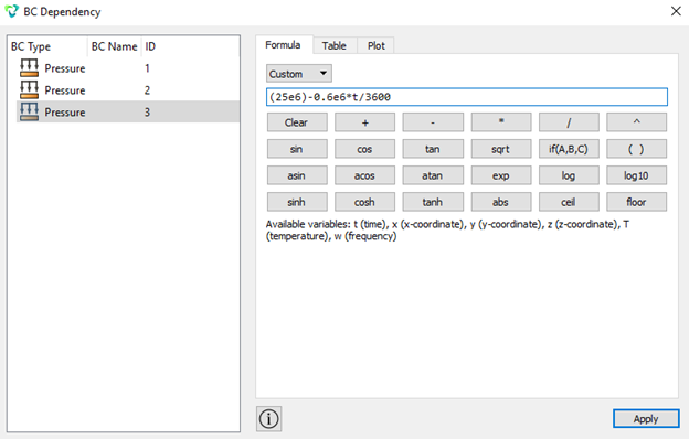
4. On the command panel, select the module for specifying Dependency BC (Mode - BC Dependency).
In the appeared BC Dependency window set the following parameters:
Click Apply.
5. Specify symmetric fixing.
On the command panel, select the boundary conditions module (Mode - Boundary Conditions, Entity - Displacement, Action - Create).
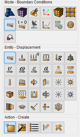
Set the following parameters:
Click Apply.
6. Similarly, set the second fixture for the line 8.
On the command panel, select the boundary conditions module (Mode - Boundary Conditions, Entity - Displacement, Action - Create).
Set the following parameters:
Click Apply.
Set the pore pressure.
On the command panel, select the boundary conditions module (Mode - Boundary Conditions, Entity - Pore Pressure, Action - Create).
Set the following parameters:
Click Apply.
1. Set the solver parameters.
On the command bar, select the calculation settings module (Mode - Calculation Settings, Calculation Settings - Transient Analysis, Transient - General).
Set the following parameters:
Check the Preload model box.
In the Models section, select the check boxes for Elasticity, Plasticity, Pore fluid transfer.
Select the check box for Set implicit scheme options.
In the field Newmark algorithm gamma, enter 0.1.
Click Apply.
Click Start Calculation.
2. In the window that appears, select the directory in which the result will be saved, and enter the file name.
3. In the case of a successful calculation, the console displays the message: Calculation finished successfully at "date" "time".
Open the file with the results. There are three ways to do that.
Click Ctrl+E.
From the main menu, select Calculation. Click Open Results.
Select Results on Command Panel (Mode - Results). Click Open results.

View the calculation results in the FidesysViewer window.
 To automatically apply changes to all filters, click
the corresponding button Apply changes to parameters automatically
on the command bar.
To automatically apply changes to all filters, click
the corresponding button Apply changes to parameters automatically
on the command bar.
Find in the standard line, the Edit color map
icon.

On the Color discretization panel, in the Number of table values field, set the value to 6.
In the top pane, select the calculation result data to display. From the first drop-down list, select Stress, and from the second - Mises.
The results of the Mises Stress are presented below (the default results
are for the last step of the calculation at the time point of 150000 s)
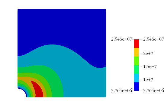
Results - Mises Stress
Similarly, we will display the remaining results.
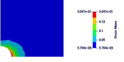
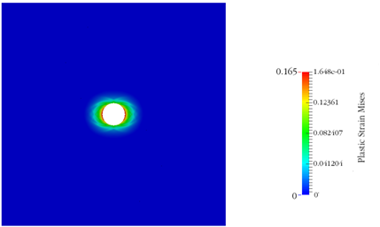
Complete the model and consider plastic deformations on the full plate. Use the Filter - Alphabetical - Flip. On the property page, in the Plane field, indicate X. Then we apply the filter Flip again to this filter, but in the Plane field, we specify Y.
On a different color scheme, the picture of the distribution of plastic
deformations may be more pronounced.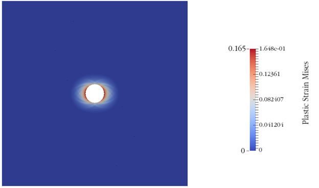
In the standard line, select Filters Alphabetical Index → Safety Factor.
Select the fields to display on the model - Safety Factor
and Coulomb-More Theory.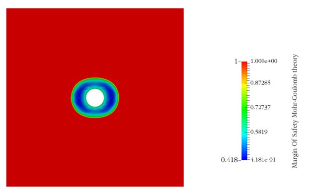
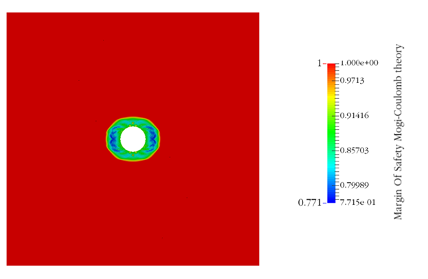
Thus, the calculation of the plastic zone around the well was made in dynamics, taking into account the pore pressure until instability appears in the form of plastic deformation bands.
Geometry creating, meshing, setting boundary conditions and materials can be performed using the console interface. Below is a link to the program code that allows you to perform the steps described above manual, you only need to specify the full path and name.