CAE Fidesys 9.0 Documentation

The Impact of Cyclic Loads on a Concrete Sample

The example considers 2 cycles of stretching-compression of a concrete sample under the action of softening. The sample material takes into account various softening curves during tension and compression.

Geometry creation

1. Create a brick.

On the command bar, select the module for constructing surface geometry (Mode - Geometry, Entity - Volume, Action - Create).

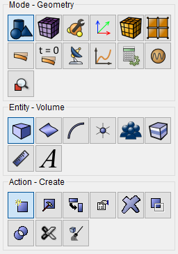
From the list of geometric primitives, select Brick.

Set the following parameters:

• X (width): 1;

• Y (height): 1;

• Z (depth): 1.

Click Apply.

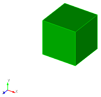
2. Move the brick.

On the command bar, select the module for constructing surface geometry (Mode - Geometry, Entity - Volume, Action - Transform).

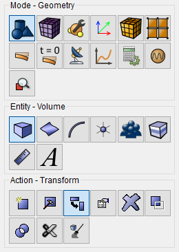
From the list select Move.

 Set the following parameters:

• Volume ID(s): 1;

• Select Method: Distance;

• X Distance: 0.5;

• Y Distance: 0.5;

• Z Distance: 0.5.

Click Apply.

Setting the material and properties of blocks

1. Specify the material.

In the command bar, select the module for specifying material properties (Mode — Material, Entity — Materials Management).

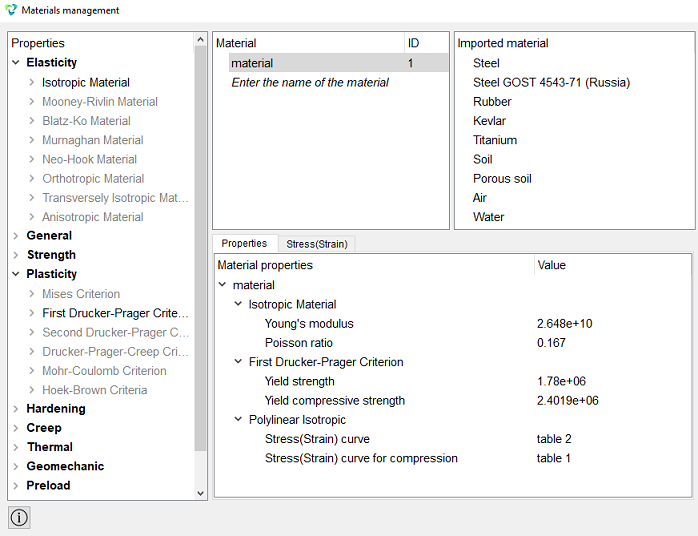
In the Materials Management window that opens, in the second column, click with the mouse on the label, specify the name of the material and write "material"

In the Materials Properties column, select the created material, and then drag the desired properties to it from the left column.

Drag the following properties:

• Young's modulus;

• Poisson ratio;

• Yield strength;

• Yield compressive strength;

• Stress(Strain) curve;

• Stress(Strain) curve for compression.

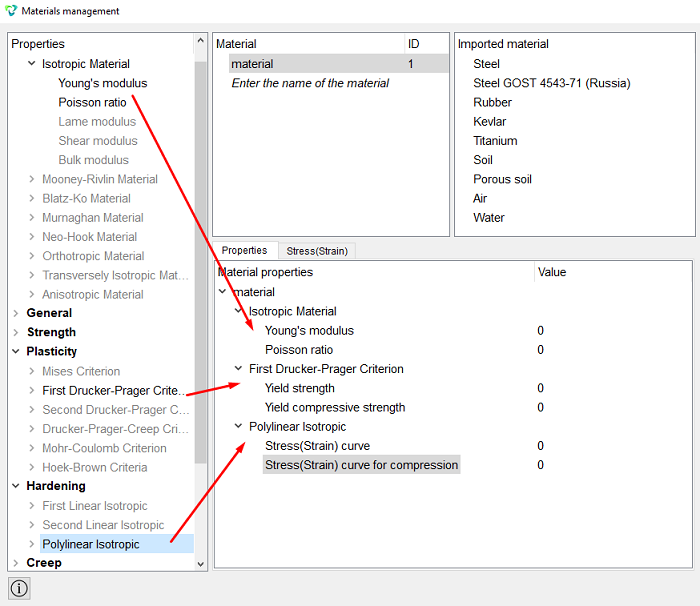
Set the required values for the material properties:

• Young's modulus: 2.648e+10;

• Poisson ratio: 0.167;

• Yield strength: 1.78e+06;

• Yield compressive strength: 2.4019e+06.

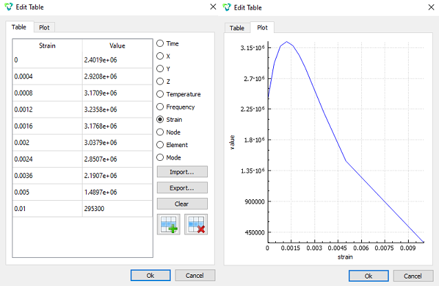
Set table values for "Stress(Strain) curve for compression":

Double click to enter the value and go to the table task

Specify that the tabular dependence will be on plastic deformation and click on to get 10 lines. Enter values:

• Strain: 0.  Value: 2.4019e+06;

• Strain: 0.0004  Value: 2.9208e+06;

• Strain: 0.0008  Value: 3.1709e+06;

• Strain: 0.0012  Value: 3.2358e+06;

• Strain: 0.0016  Value: 3.1768e+06;

• Strain: 0.002  Value: 3.0379e+06;

• Strain: 0.0024  Value: 2.8507e+06;

• Strain: 0.0036  Value: 2.1907e+06;

• Strain: 0.005  Value: 1.4897e+06;

• Strain: 0.01  Value: 295300.

Click ok.

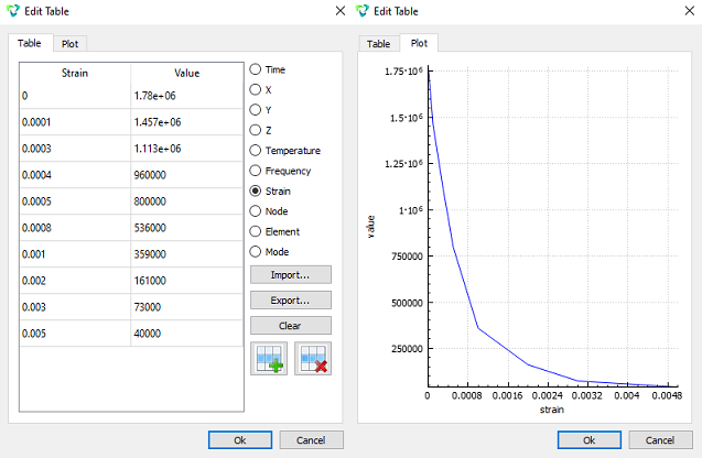
Set table values for "Stress(Strain) curve":

Double click to enter the value and go to the table task

Specify that the tabular dependence will be on plastic deformation and click on to get 10 lines. Enter values:

• Strain: 0.  Value: 1.78e+06;

• Strain: 0.0001  Value: 1.457e+06;

• Strain: 0.0003  Value: 1.113e+06;

• Strain: 0.0004  Value: 960000;

• Strain: 0.0005  Value: 800000;

• Strain: 0.0008  Value: 536000;

• Strain: 0.001  Value: 359000;

• Strain: 0.002  Value: 161000;

• Strain: 0.003  Value: 73000;

• Strain: 0.005  Value: 40000.

Click ok.

Click Apply.

Close the Materials management window.

2. Create a block.

On the command bar, select the block management module (Mode - Blocks, Entity - Block, Action - Add).

Set the following parameters:

• Entity List: Volume;

• Entity ID(s): 1.

Click Apply.

3. Set the block parameters.

On the command bar, select the block management module (Mode - Blocks, Entity - Block, Action - Block properties/parameters).

Set the following parameters:

• Block ID(s): 1;

• Category: Solid;

• Material: material;

• Coordinate System: Global Cartesian;

• Order: 1.

Click Apply.

Meshing

1. Set the mesh split.

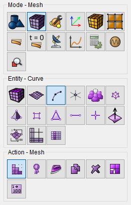
On the command bar, select the mesh module (Mode - Mesh, Entity - Curve, Action - Mesh).

Set the following parameters:

• Select Curves: all;

• From the drop-down list select Equal;

• Select the radio button Interval;

• Interval: 1.

Click Apply Size.

2. Create a mesh.

On the command bar, select the volume mesh module (Mode - Mesh, Entity - Volume, Action - Mesh).

From the list of actions, select Automatically Calculate.

Set the following parameters:

• Select Volumes: 1.

Click Mesh.

Setting boundary conditions

1. Fix the model in the movements.

On the command panel, select the boundary conditions module (Mode - Boundary Conditions, Entity - Displacement, Action - Create).

Set the following parameters:

• Entity List: Surface;

• Entity ID(s): 3;

• Degrees Of Freedom: Y-Translation Disp;

• DOF Value: 0.

Click Apply.

2. Fix the model in the movements.

On the command panel, select the boundary conditions module (Mode - Boundary Conditions, Entity - Displacement, Action - Create).

Set the following parameters:

• Entity List: Surface;

• Entity ID(s): 2;

• Degrees Of Freedom: Z-Translation Disp;

• DOF Value: 0.

Click Apply.

3. Fix the model in the movements.

On the command panel, select the boundary conditions module (Mode - Boundary Conditions, Entity - Displacement, Action - Create).

Set the following parameters:

• Entity List: Surface;

• Entity ID(s): 4;

• Degrees Of Freedom: X-Translation Disp;

• DOF Value: 0.

Click Apply.

4. Fix the model in the movements.

On the command panel, select the boundary conditions module (Mode - Boundary Conditions, Entity - Displacement, Action - Create).

Set the following parameters:

• Entity List: Surface;

• Entity ID(s): 5;

• Degrees Of Freedoms: Y-Translation Disp;

• DOF Value: 0.

Click Apply.

Setting time dependency of boundary conditions

1. Set the dependency to move.

On the command panel, select the module for specifying Dependency BC (Mode - BC Dependency).

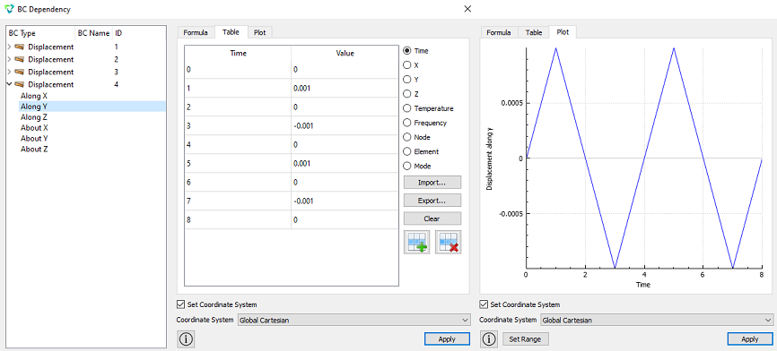
Click on Displacement 4 and specify that the tabular dependence will be on time. Click on to get 9 lines. Enter values:

• Time: 0.  Value: 0;

• Time: 1  Value: 0.001;

• Time: 2  Value: 0;

• Time: 3  Value: -0.001;

• Time: 4  Value: 0;

• Time: 5  Value: 0.001;

• Time: 6  Value: 0;

• Time: 7  Value: -0.001;

• Time: 8  Value: 0.

Starting calculation

1. Set the type of problem you need to solve.

On the command bar, select the calculation settings module (Mode - Calculation Settings, Calculation Settings - Static, Static - General).

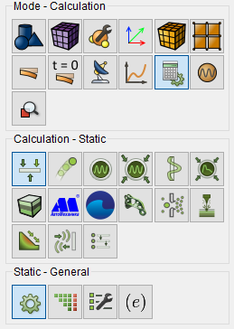
Select:

• Dimensions: 3D;

• Model: Elasticity;

• Model: Plasticity;

• Set static load steps count;

• Load steps count: 8;

• Set nonlinear solver options;

• Start load substeps: 101;

• Min load substeps: 100;

• Max load substeps: 1000000;

• Max iterations: 1000;

• Tolerance: 1e-6;

• Target iterations: 5.

Click Apply.

Click Start Calculation.

2. In the window that appears, select the directory where the result will be saved and enter the file name.

3. In the case of a successful calculation, the console displays the message: Calculation finished successfully at "date" "time".

Results analysis

1. Open the file with the results. There are three ways to do that.

• Click Ctrl+E.

• From the main menu, select Calculation. Click Open Results.

• Select Results on Command Panel (Mode - Results). Click Open results.

The FidesysViewer window will appear, in which you can view the calculation results.

Select a point on the model using the button Select Points On and apply the filter Plot Selection Over Time.

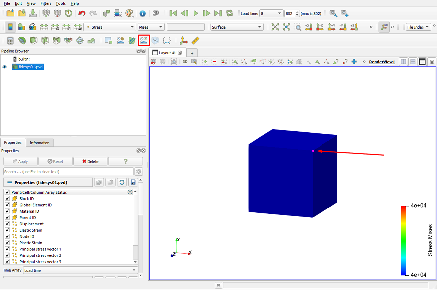
As a field to display on the chart, select Stress_Mises. As a result, the necessary graph of the dependence of stress intensity on time will be displayed on the right side of the screen:

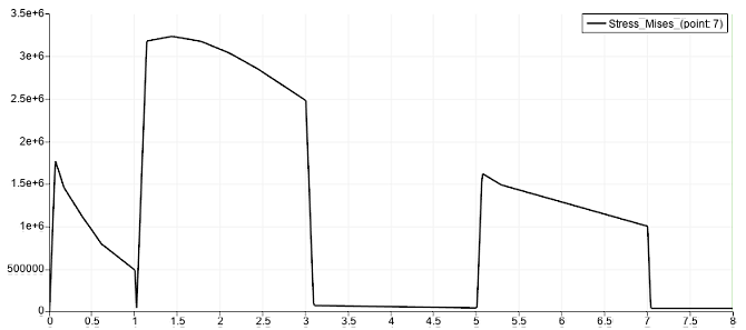
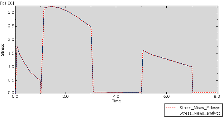
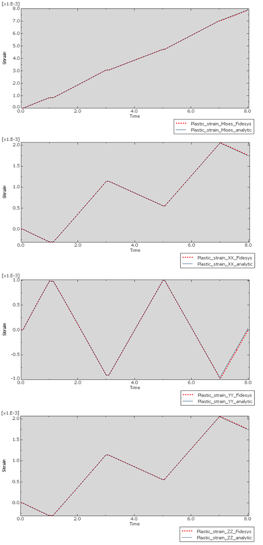
Comparison with an analytical solution:

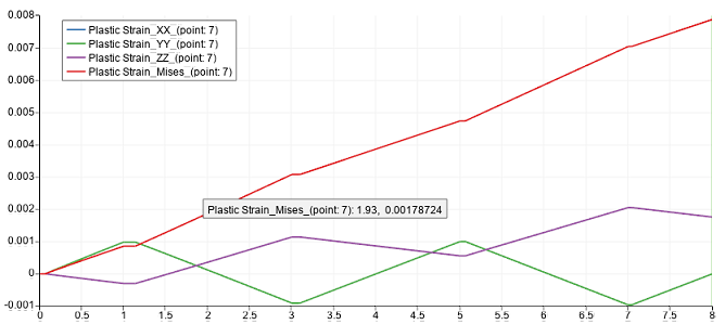
Next, in the display field, select Plastic Strain_XX, Plastic Strain_YY, Plastic Strain_ZZ, Plastic Strain_Мизес. As a result, graphs of the dependences of the intensity and components of the plastic strain tensor on time will be displayed:

Comparison with an analytical solution:

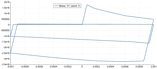
In the filter properties, change the X Array Name, to do this, select Strain_YY from the drop-down list. Then, in the display field, select Stress_YY. As a result, the necessary graph of the dependence of normal stress on normal deformation will be displayed:

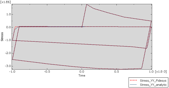
Comparison with an analytical solution:

Using Console Interface

Geometry creating, meshing, setting boundary conditions and materials can be performed using the console interface. Below is a link to the program code that allows you to perform the steps described above manual, you only need to specify the full path and name.

cyclic_stretching_compression_softening