Search the documentation
Enter at least 2 characters
Enter at least 2 characters
 |
CAE Fidesys 9.0 Documentation |
CAE Fidesys allows you to upload solution results in SEG-Y format. This example considers the propagation of seismic waves in the ground based on the Lamb problem for a 2D case. The procedures for setting receivers, saving and subsequent analysis of data in the SEG-Y format are demonstrated.
The model is a part of the plane (xy), a point force is applied to vertex. Non-reflective boundary conditions are applied.
1. Create a square plate.
On the command bar, select the module for constructing surface geometry (Mode - Geometry, Entity - Surface, Action - Create).
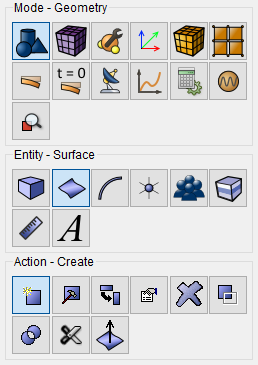
From the list of geometric primitives, select Rectangle.
Set block sizes:
Width: 1000;
Location: ZPlane.
Click Apply.
2. Due to symmetry, we consider half of the model.
On the command bar, select the module for constructing surface geometry (Mode - Geometry, Entity - Surface, Action - Webcut).
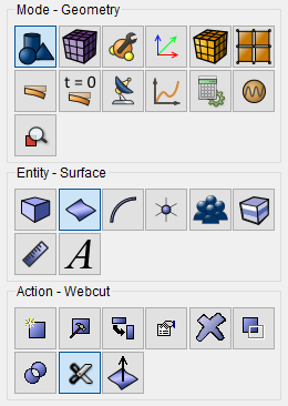
From the list of possible kind of webcuts, select Coordinate Plane.
Set the following parameters:
Body ID(s): 1 (the body to be cut);
Cut: YZ;
Offset Value: 0.
Click Apply.
Do the same, but in the ZX plane.
Body ID(s): 1 (the body to be cut);
Cut: ZX;
Offset Value: 0.
Click Apply.
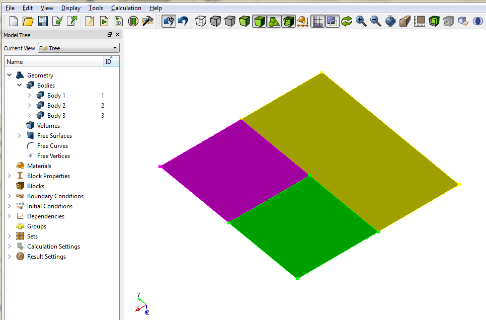 As a result, the original Body 1 in the Model Tree
will be divided into three bodies (Body 1, Body 2 and Body 3).
As a result, the original Body 1 in the Model Tree
will be divided into three bodies (Body 1, Body 2 and Body 3).
3. Delete Surface 3.
On the command bar, select the module for constructing surface geometry (Mode - Geometry, Entity - Surface, Action - Delete).
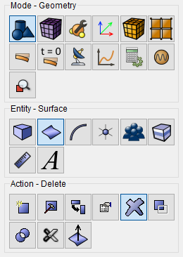
Set the parameters:
Surface ID (s): 3.
Click Apply.
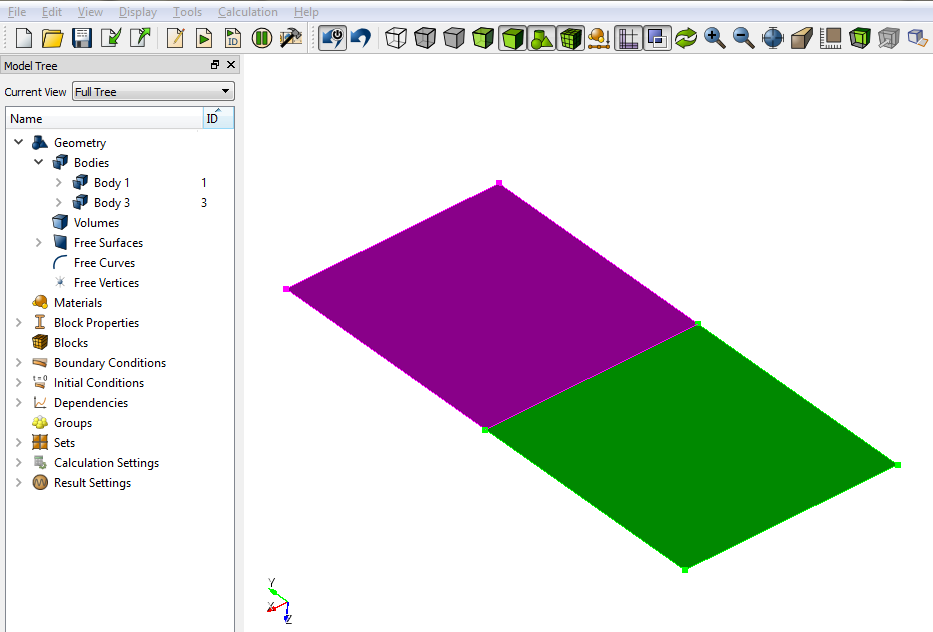
4. Rotate the model.
On the command bar, select the module for constructing surface geometry (Mode - Geometry, Entity - Surface, Action - Transform).
Select Rotate in the list of operations.
Set the following parameters:
Surface ID(s): 4 5;
Tick the box: Include Merged;
Angle: -90;
Rotate About: Z-Axis.
5. Cut the model.
On the command bar, select the module for constructing surface geometry (Mode - Geometry, Entity - Surface, Action - Webcut).
From the list of possible kind of webcuts, select Coordinate Plane.
Set the following parameters:
Body ID(s): 3 1;
Cut: ZX;
Offset Value: -250.
Click Apply.
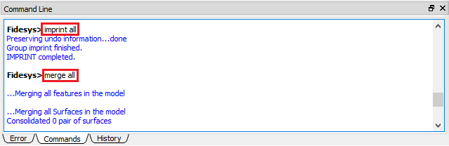
6. Imprint and merge the following commands on the command line:
imprint all;
merge all.
1. Make sure that in the main menu settings (Tools - Options — Mesh Defaults) Default Element Type Hex/Quad is selected.
2. On the command bar, select the surface mesh module (Mode - Mesh, Entity - Surface, Action - Intervals).
Specify the degree of mesh refinement:
Approximate Size;
Select Surfaces: all;
Approximate Size: 7.
Click Apply Size.
Click Mesh.
1. In the command bar, select the module for specifying material properties (Mode - Material, Entity - Materials Management).

In the opened widget Material Management in the middle column specify the material name. In the properties column, open the Elasticity list and drag Isotropic Material to the Material Properties column, then in the left column go to the section and drag General → Density and Plasticity → Second Drucker-Prager Criterion. Set the following parameters:
Young's modulus: 2e+08;
Poisson ratio: 0.3;
Density: 1900;
Cohesion: 29000;
Internal friction angle: 20;
Dilatancy angle: 10.
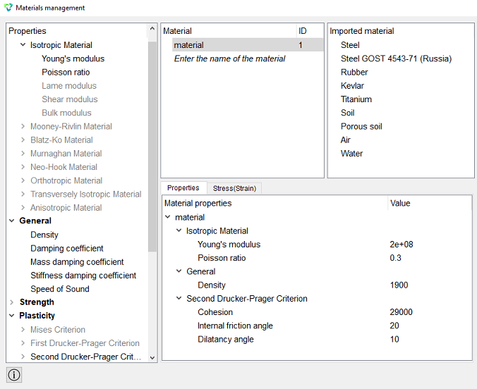
Click Apply.
Close the Materials management window.
2. Create a block of one material type.
On the command bar, select the block management module (Mode - Blocks, Entity - Block, Action - Add).

Set the following parameters:
Block ID: 1;
Entity List: Surface;
Entity ID(s): All.
Click Apply.
3. Set the block parameters.
On the command bar, select the block management module (Mode - Blocks, Entity - Block, Action - Block properties/parameters).

Set the following parameters:
Block ID(s): 1;
Category: Plane;
Material: material;
Coordinate System: Global Cartesian;
Order: 3.
Click Apply.
1. Set non-reflective boundary conditions.
On the command panel, select the boundary conditions module (Mode - Boundary Conditions, Entity – Absorbing Condition, Action - Create).
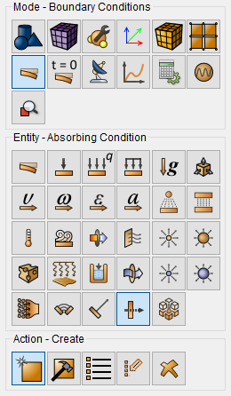
Set the following parameters:
Entity List: Curve;
Entity ID(s): 28 24 13 15 19 21 (separated by spaces).
Click Apply.
2. Set the force.
On the command panel, select the boundary conditions module (Mode - Boundary Conditions, Entity - Force, Action - Create).
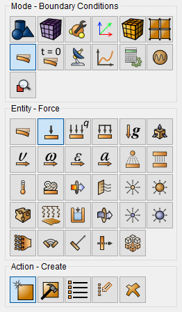
Set the following parameters:
Force Entity List: Vertex;
Entity ID(s): 10;
Force: 1;
Direction: 0 -1 0 (space separated).
Click Apply.
1. Create a formula 1 for strength 1.
On the command panel, select the module for specifying Dependency BC (Mode - BC Dependency).
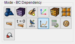
Click Force 1 and choose Formula panel in the right. Then choose Berlage and set the following parameters:
Select the flag Formula: Berlage;
Amplitude: 1e+8;
Frequency: 10.
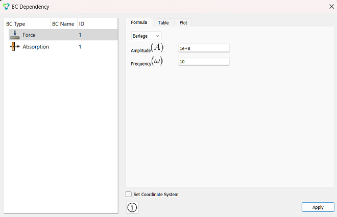
Click Apply. Close the BC Dependency window.
1. Create receivers on curve 16 along all directions.
On the command panel, select module for setting receivers (Mode - Receivers, Operation - Create).
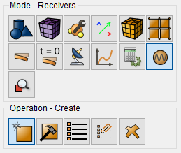
From the drop-down list, select the fields whose data you want to save in SEG-Y format.
Set the following parameters:
Entity List: Curve;
Entity ID(s): 16;
Displacement;
Variables: All.
Click Apply.
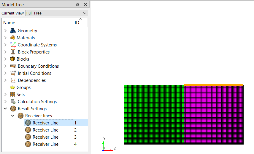
Repeat all the steps with the same parameters for each field in the drop-down list (velocity, principal stress).
The receiver lines are highlighted on the model in yellow when clicked in the corresponding section of the Model Tree.
1. Set the type of problem you want to solve.
On the command bar, select the calculation settings module (Mode - Calculation Settings, Calculation Settings - Transient Analysis, Transient - General).
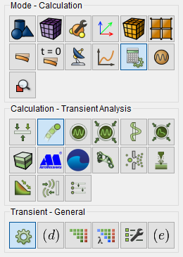
Set the following calculation parameters:
Dimension: 2D;
Method: Full solution;
Scheme: Explicit;
Max time: 3;
Steps count: 2025;
Preload model: uncheck.
Click Apply.
2. Go to the output fields settings section.
On the command bar, select the calculation settings module (Mode - Calculation Settings, Calculation Settings - Transient Analysis, Transient - Output Fields).
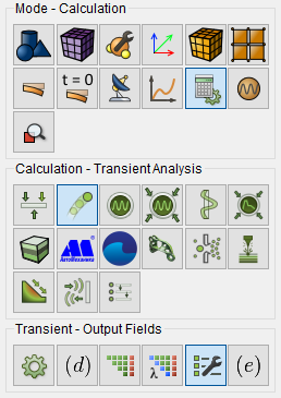
Specify:
Save Results: Every 135 Steps.
Click Apply.
Click Start Calculation.
3. In the window that appears, select the directory in which the result will be saved, and enter the file name.
4. In the case of a successful calculation, the console displays the message: Calculation finished successfully at "date" "time".
1. Open the file with the results. There are three ways to do that.
Click Ctrl+E.
From the main menu, select Calculation. Click Open Results.
Select Results on Command Panel (Mode - Results). Click Open results.

2. To analyze the results, go to the FidesysViewer.
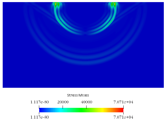
3. On the top bar, select the required result data to display. From
the first drop-down list, select Stress, from the second
- Mises.
4. Set the step 1 in the step viewer panel. You should see the plate
image in the initial state. Next, click on Play  .
You should see the propagation of stress over time.
.
You should see the propagation of stress over time.
5. Open the saved data in SEG-Y format.
To do this, go to Menu - File - Open.
In the drop-down list of file types, select SEG-Y Files (* .sgy, * .segy).
Specify the file to view test_Vy.sgs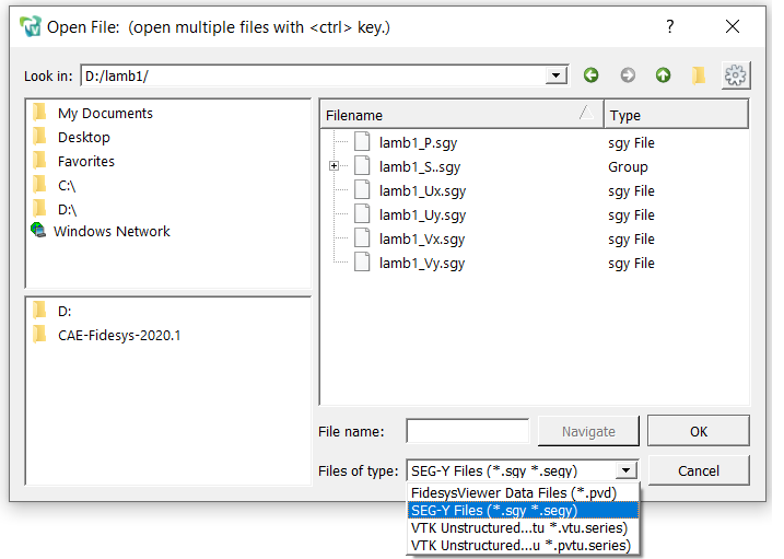
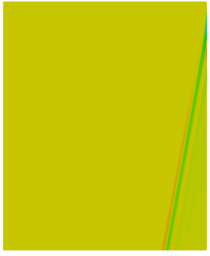
Set the viewing direction along the Y axis.

The calculation results for displacement Uy in the SEG-Y format are visualized in the field of visualization.
Geometry creating, meshing, setting boundary conditions and materials can be performed using the console interface. Below is a link to the program code that allows you to perform the steps described above manual, you only need to specify the full path and name.