Search the documentation
Enter at least 2 characters
Enter at least 2 characters
 |
CAE Fidesys 9.0 Documentation |
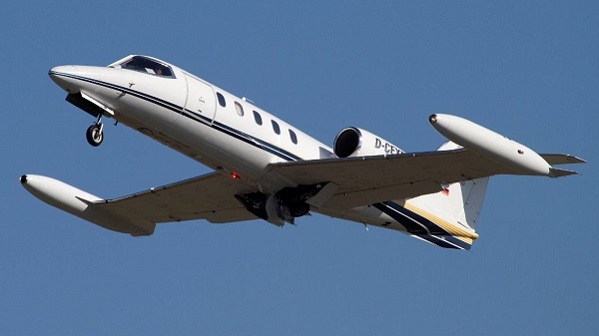
Learjet 35 (LJ35) — jet administrative aircraft production Learjet Business Class companies (Learjet 35 and Learjet 36 versions) and the US Air Force C-21A military transport aircraft.
The aircraft is equipped with two Garrett TFE731 turbofan engines. The cabin of the aircraft can accommodate 6-8 passengers. In the Learjet 36 version , the aircraft it has a reduced passenger compartment for placement in the tail section fuselage of additional fuel tanks.
The engines are mounted in nacelles on the sides of the rear fuselage. The wings are equipped with single-slit flaps. Wing fuel tanks are located in the wingtips, which distinguishes the design of the aircraft from other aircraft.
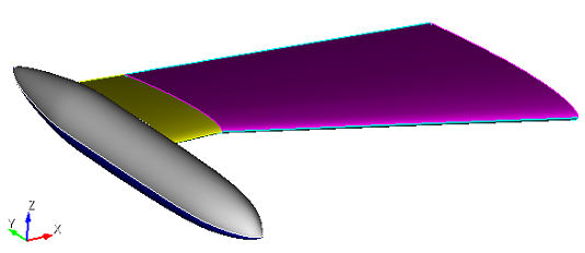
Static calculation of laminate shells. The problem is considered by example calculation of the wing of the aircraft together with the fuel tank.
1. Download the model from the link: Download geom_acis.sat. If you cannot download the model, right-click on its name and select Save target as.... Then specify the folder where you want to go. place it.
The file can also be found in the folder C:\Program Files\Fidesys\CAE-Fidesys-9.0\preprocessor\bin\help\fidesys_example_tutorials\TestsFromHelp\models and select the specified model.
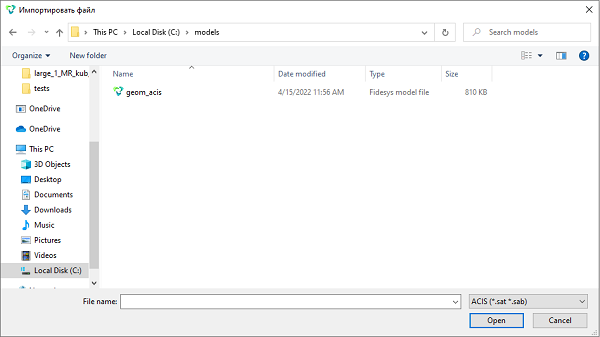
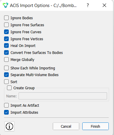
2. Import the model. In the top line, select (Menu — File — Import). Specify the path to the geom_acis.sat file. In the window that appears set the import settings:
Ignore free curves;
Ignore free vertices;
Heal on import;
Convert free surfaces to bodies;
Separate multi-volume bodies.
3. Fuse the surfaces.
On the command bar, select the module for constructing surface geometry (Mode — Geometry, Entity – Surface, Action – Merge).
From the pop-up list, select: Merge.
Set the following parameters:
Surface ID(s): all.
Click Apply.
4. Merge the curves.
On the command bar, select the module for constructing geometry (Mode — Geometry, Entity – Curve, Action – Merge).
From the pop-up list, select: Merge.
Set the following parameters:
Curve ID(s): all.
Click Apply.
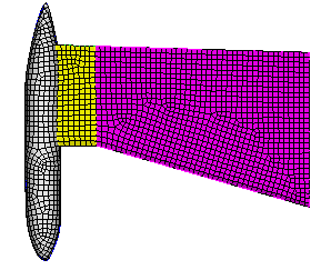
1. Create an automatic generation on the surface of an irregular mesh of quadrilaterals. At the command prompt, type: surface all scheme pave.
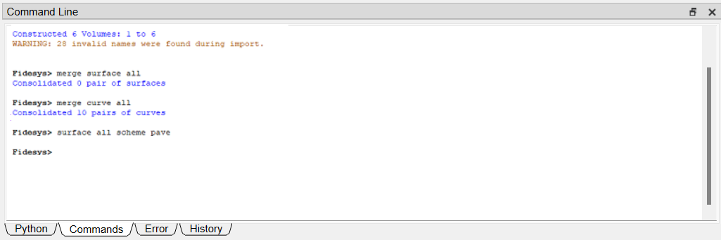
2. On the command bar, select the surface mesh module (Mode — Mesh, Entity – Surface, Action – Intervals).
From the pop-up list, select: Automatic Sizing.
Select Surfaces: all;
Move the Auto Factor slider to 1.
Click Apply Size.
Click Mesh.
1. Set a new coordinate system.
On the command bar, select (Mode — Coordinate System, Coordinate System — Create).
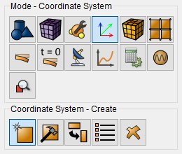
Set the following parameters:
Type: Cartesian;
Оrigin Entity: Vertex;
Entity ID: 12;
Direction 1 Entity: Vertex;
Entity ID: 1;
Direction 2 Entity: Vertex;
Entity ID: 11.
Click Apply.
2. Set another coordinate system. On the command bar, select (Mode — Coordinate System, Coordinate System — Create).
Set the following parameters:
Type: Cartesian;
Оrigin Entity: Vertex;
Entity ID: 18;
Direction 1 Entity: Vertex;
Entity ID: 17;
Direction 2 Entity: Vertex;
Entity ID: 1.
Click Apply.
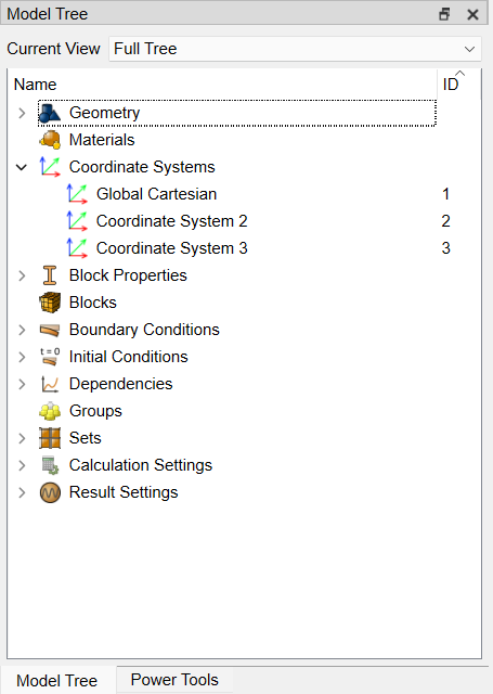
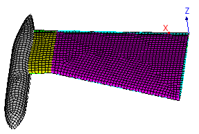
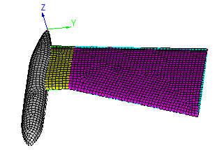
In the entity tree, select Coordinate System. Then check that you have 3 coordinate systems. Click on each one and see where they are are located.
1. Specify the material.
In the command bar, select the module for specifying material properties (Mode — Material, Entity— Materials Management).

In the column "Imported material", double-click on Kevlar.
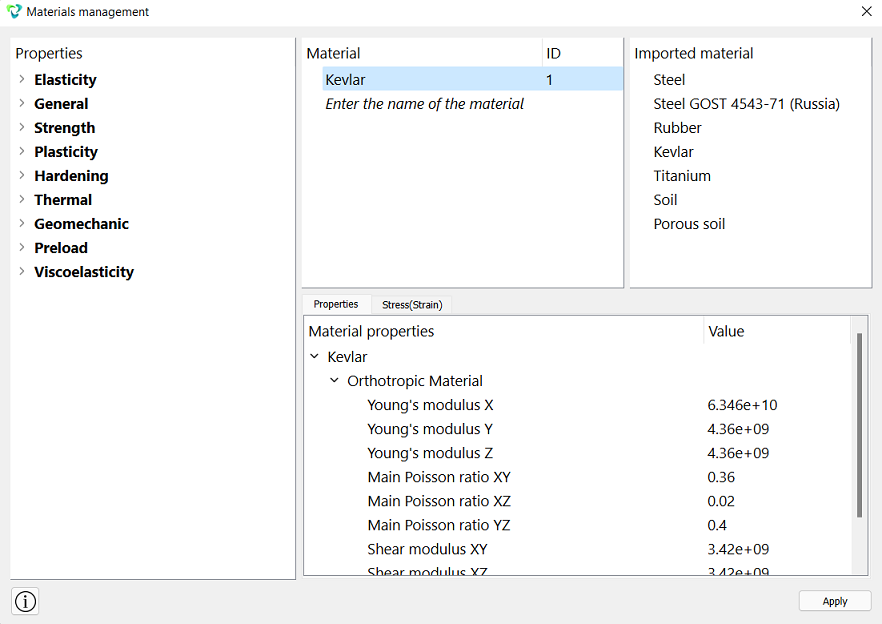
Click Apply.
Close the Materials management window.
2. Change the material properties.
In the command bar, select the module for specifying material properties (Mode — Material, Entity — Materials Management).
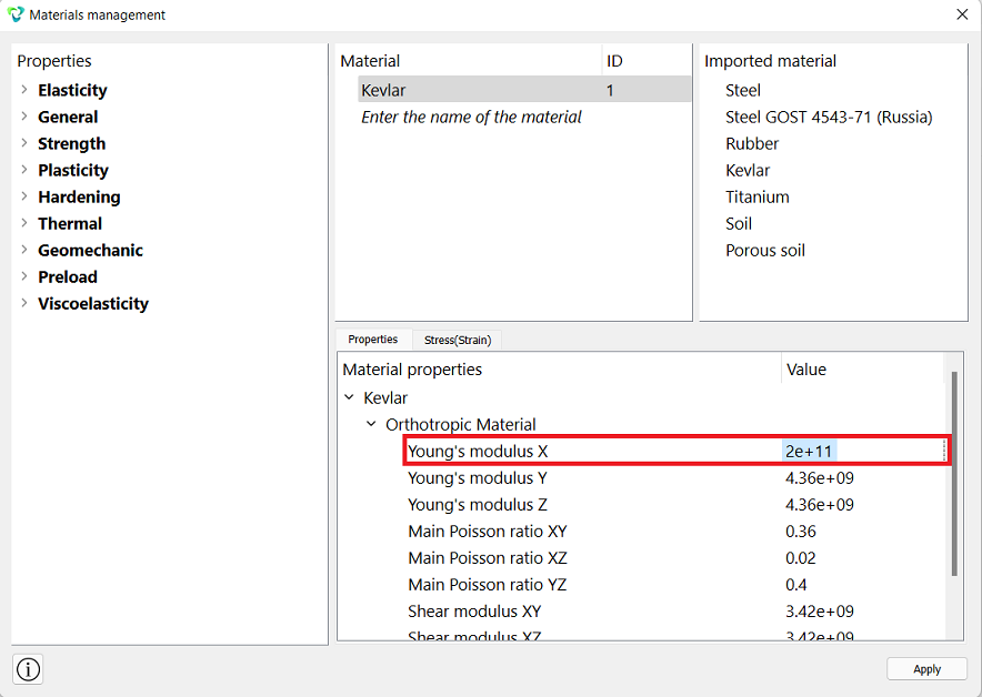
In the column "Material" click on Kevlar.
In the "Properties" column materials"change the value Young's Modulus X = 2e+11.
Click Apply.
3. Change the name of the material.
In the command bar, select the module for specifying material properties (Mode — Material, Entity— Materials Management).
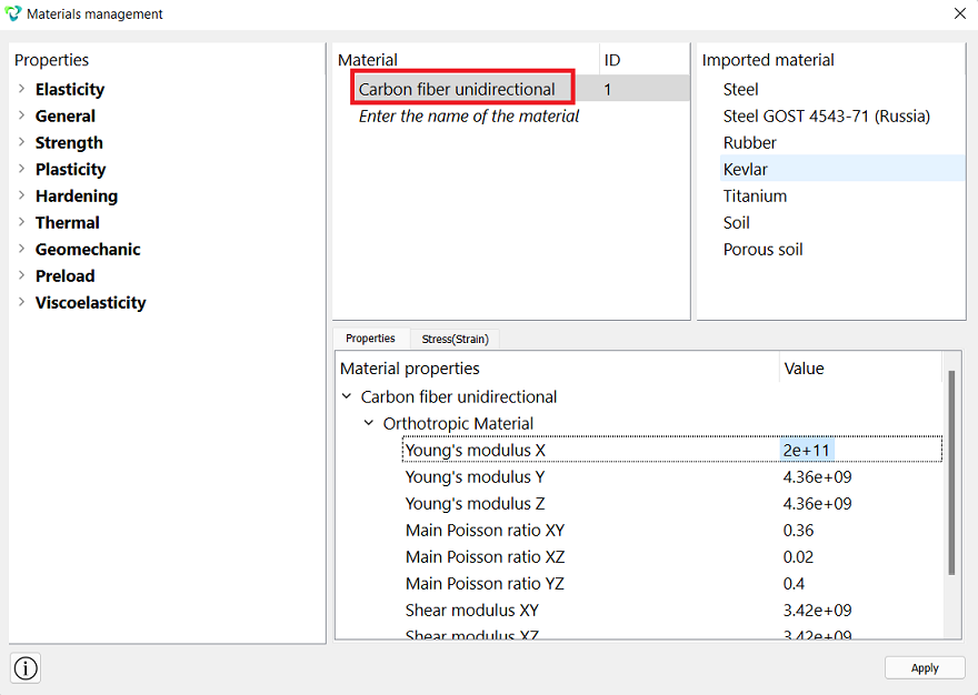
In the "Material" column, double-click on Kevlar. Change name on Carbon fiber unidirectional.
Click Apply.
4. Create a block for the wing.
On the command bar, select the block management module (Mode — Blocks, Entity — Block, Action — Add).

Set the following parameters:
Entity List : Surface;
Entity ID(s): all.
Click Apply.
5. Remove the surfaces belonging to the fuel tank of the aircraft from the block.
On the command bar, select the block management module (Mode — Blocks, Entity — Block, Action — Modify).
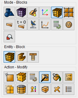
Set the following parameters:
Click Apply.
6. Create a block for the fuel tank.
On the command bar, select the block management module (Mode — Blocks, Entity — Block, Action — Add).
Set the following parameters:
Entity List: Surface;
Entity ID(s): 6 5;
Click Apply.
7. Set the parameters for the first block.
On the command bar, select the block management module (Mode — Blocks, Entity — Block, Action — Block properties/parameters).

Set the following parameters:
Block ID(s): 1;
Category: Shell;
Coordinate System: Coordinate System 2;
Order: 1.
Set the shell properties, to do this, click on the button  .
.
Set the following options:
Thickness: 0.002;
Material: Carbon fiber Unidirectional;
Angle: -30;
Click on the buttonAdd a line  and add properties for the second layer. Set shell properties:
Thickness: 0.002;
Material: Carbon fiber Unidirectional;
Angle: 30;
Eccentricity: 0.5.
Click Apply. Then close the properties.
Click Apply.
8. Set the parameters for the second block.
On the command bar, select the block management module (Mode — Blocks, Entity — Block, Action — Block properties/parameters).
Set the following parameters:
Block ID(s): 2;
Category: Shell;
Coordinate System: Coordinate System 3;
Material: Carbon fiber Unidirectional;
Order: 1;
ID : 1.
Click Apply.
1. Since the wing of the aircraft is attached to its main part, secure the separation point.
On the command panel, select the boundary conditions module (Mode — Boundary Conditions, Entity — Displacement, Action — Create).
Set the following parameters:
Entity List: Curve;
Entity ID(s): 11 15;
Degrees of Freedom: X-Translation Disp, Y-Translation Disp, Z-Translation Disp;
DOF Value: 0.
Click Apply.
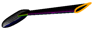
2. Set the pressure for the lower part of the model.
On the command panel, select the boundary conditions module (Mode — Boundary Conditions, Entity — Pressure, Action — Create).
Set the following parameters:
Pressure Entity List: Surface;
Entity ID(s): 4 1 5;
Magnitude Value: 1e4.
Click Apply.
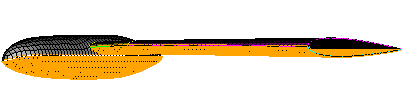
3. Set the gravitational force.
On the command panel, select the boundary conditions module (Mode — Boundary Conditions, Entity — Gravity, Action — Create).
Set the following parameters:
Entity List: Global;
Directions: Z: -9.81.
Click Apply.
1. Specify the type of task you want to solve.
On the command bar, select the calculation settings module (Mode — Calculation Settings, Calculation Settings — Static, Static — General).
Select:
Dimensions: 3D;
Model: Elasticity.
On the Command Bar, click Apply and then Start Calculation.
3. In the window that appears, select the directory where the result will be saved
4. In the case of a successful calculation, the console displays the message: Calculation finished successfully at "date" "time".
1. Open the file with the results. There are three ways to do that.
Click Ctrl+E.
From the main menu, select Calculation. Click Open Results.
Select Results on Command Panel (Mode - Results). Click Open results.

A window will appear FidesysViewer, in which you can read with the results of the calculation.
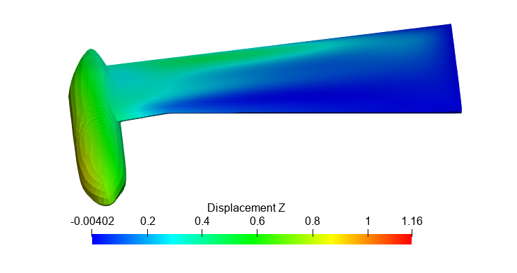
2. In the upper panel, select the calculation result data to display. From the first drop-down list, select Displacement, from the second – Z.
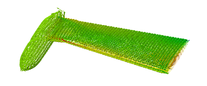
3. Check the direction of each shell layer separately. In the top row select (Menu — Filters — Alphabetical index — Construct a vector field).
In the Properties, select:
Field Type: Arrow;
Orientation → Direction array: Local Coordinate System Vector X (shell layer 1)
Scale → Direction array: Local Coordinate System Vector X (shell layer 1)
Click Apply.
On the top bar select Stress (shell layer 1), XX
 .
.
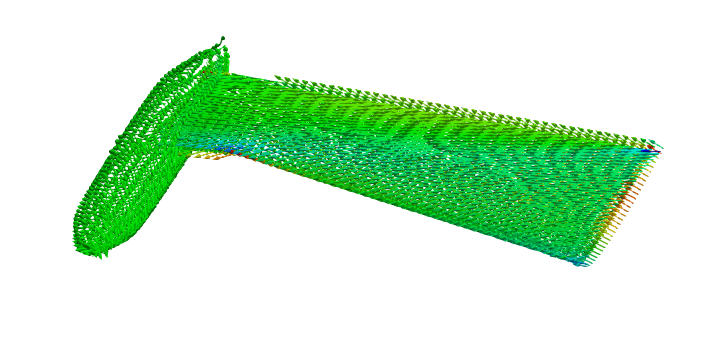
4. Check the direction of each shell layer separately. In the top row select (Menu — Filters — Alphabetical index — Construct a vector field).
In the Properties, select:
Field Type: Arrow;
Orientation → Direction array: Local Coordinate System Vector X (shell layer 2)
Scale → Direction array: Local Coordinate System Vector X (shell layer 2)
Click Apply.
On the top bar select Stress (shell layer 2), XX
 .
.
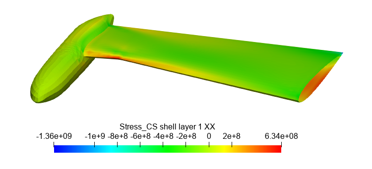
5. Apply a filter "Coordinate systems" to display results in the coordinate system of each layer. In the top row select (Menu — Filters — Alphabetical index — Coordinate systems).
In the Properties, select:
Uncheck the boxes "Spherical coordinates" и "Cylindrical coordinates";
Check the boxes "Shell layer coordinate systems".
Click Apply.
From the first drop-down list, select Stress_СS shell layer 1, from the second – XX.
Geometry creating, meshing, setting boundary conditions and materials can be performed using the console interface. Below is a link to the program code that allows you to perform the steps described above manual, you only need to specify the full path and name.