Search the documentation
Enter at least 2 characters
Enter at least 2 characters
 |
CAE Fidesys 9.0 Documentation |
Approximation of this partial differential equation with given boundary
and initial conditions is performed using an implicit finite-volume scheme.
Uses a regular three-dimensional grid of box cells with indexes  ,where IM, JM, KM - number of cells along each
coordinate axis.
,where IM, JM, KM - number of cells along each
coordinate axis.  - coordinates
of cell centers.
- coordinates
of cell centers.
Cell volume integration leads to the following scheme:
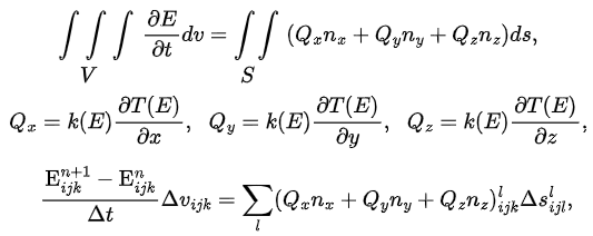
where l is the cell side index,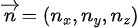 — unit vector of the outer normal. In the case of a box mesh, each component
 can be 0, +1, or -1,
and exactly two of the three components are always 0 for either side of
the cell.
can be 0, +1, or -1,
and exactly two of the three components are always 0 for either side of
the cell.
As noted earlier, the equation is nonlinear. To solve it, the predictor-corrector approach is used. At the predictor step, we approximate the flows on the right side, indicated by the superscript P, using the values k and dT/dE at the current time step n, but use the enthalpy values at the next (intermediate) step n+1/2:
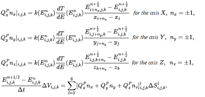
In the corrector step, we approximate the flows on the right side, indicated by the superscript C, using the values k and dT/dE at the intermediate time step n+1/2, which may differ from the values at the time step n, while the enthalpy values are taken at the next time step n+1:
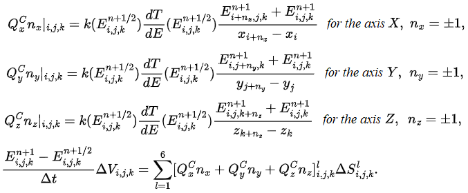
Here  — cell volume
(i, j, k);
— cell volume
(i, j, k);  — area of
the l-th cell side (i, j, k). For cells at the boundary of the calculated
area, flows are known from boundary conditions.
— area of
the l-th cell side (i, j, k). For cells at the boundary of the calculated
area, flows are known from boundary conditions.
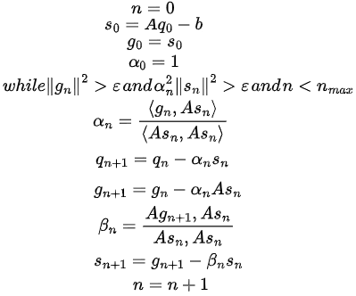
The described implicit scheme, which allows a significantly longer time step Δ t than the stability condition for an explicit scheme allows, leads to the need to solve large sparse systems of linear algebraic equations of the form Aq = b. Here, the unknown vector q denotes all unknown enthalpy values of E, the known vector of the right-hand side b depends on the known enthalpy values at the current time step, and A is a sparse system matrix. An iterative method can be used to solve this system. One of its advantages are that there is no need to explicitly shape matrix: it is enough to be able to effectively calculate the product of the matrix by vector. We used a matrix-free iterative method of conjugate gradients for asymmetric matrices. Its computational formulas have the form (with additional vectors s and g), where the angle brackets 〈.,. 〉 denote the dot product: