Search the documentation
Enter at least 2 characters
Enter at least 2 characters
 |
CAE Fidesys 9.0 Documentation |
S.P. Timoshenko, J.M Manages “Theory of elastic stability” second edition. Dunod, 1966, 500 pages
We solve the problem of cylindrical shell buckling under the pressure uniformly distributed over the entire surface.
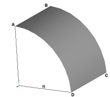
The picture represents a geometric model of the problem: R = 2 m, L = 2 m, thickness h = 0.02 m. Due to the symmetry of the problem, the ¼ part of the cylinder is regarded. Constraints on the lines AB and CD are due to the conditions of symmetry; a uniformly distributed load on the surface is ABCD q = 1 kPa. The material parameters are E = 200 GPa, ν = 0.3.
It is necessary to compare the first three critical values.
1. Create a cylinder with radius of 2 m and length of 2 m.
On the command bar, select the module for constructing volume geometry (Mode — Geometry, Entity — Volume, Action — Create).
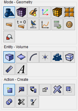
Select Cylinder in the list of geometric elements.
Specify the cylinder dimensions:
Height: 2;
Cross section: Circular;
Radius: 2.
Click Apply.
2. Get the cylindrical shell out of the volume ric cylinder.
On the command bar, select the module for constructing volume geometry (Mode — Geometry, Entity — Volume, Action — Delete).
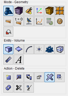
Set the following parameters:
Volume ID(s): 1;
Put a tick against Keep Lower Geometry.
Click Apply.
As a result, three plane bodies (Body 1, Body 2, Body 3) are obtained. This will be displayed in the Model Tree.
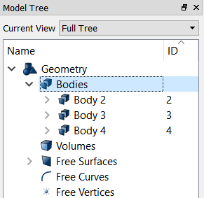
3. Delete side surfaces Body 3 and Body 4.
On the command bar, select the module for constructing volume geometry (Mode — Geometry, Entity — Volume, Action — Delete).
Set the following parameters:
Volume ID(s): 2 3.
Click Apply.
As a result, only the lateral cylindrical shell of 2 m radius and 2 m high will remain of the initial volume.
4. Leave a quarter of a shell (symmetry of the problem).
On the command bar, select the module for constructing surface geometry (Mode — Geometry, Entity — Surface, Action — Webcut).
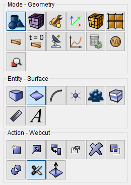
Select Coordinate Plane in the list of possible webcut types.
Set the following parameters:
Body ID(s): 2 (the surface to be webcut);
Webcut with Plane: YZ;
Offset Value: 0;
Imprint.
Click Apply.
Do the same for the ZX Plane:
Body ID(s): 2 (the volume to be webcut);
Webcut with Plane: ZX;
Offset Value: 0;
Imprint.
Click Apply.
As a result, the original volume in the Model Tree is split into three (Body 2, Body 5 and Body 6).
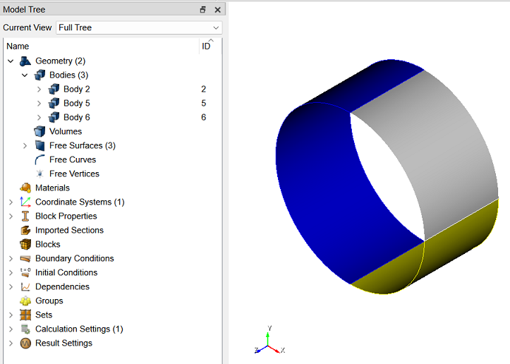
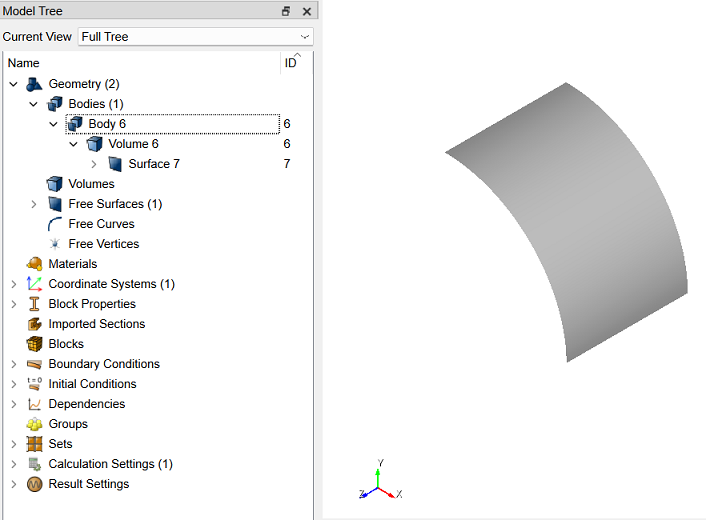
Delete the bodies 2 and 5. To do this select these bodies in the Model Tree holding down the Ctrl key and click Delete in contextual menu. As a result, a quarter of the original shell is left (Body 6):
1. Create a quadrangular mesh.
On the command bar, select the surface mesh module (Mode — Mesh, Entity — Surface, Action — Intervals).
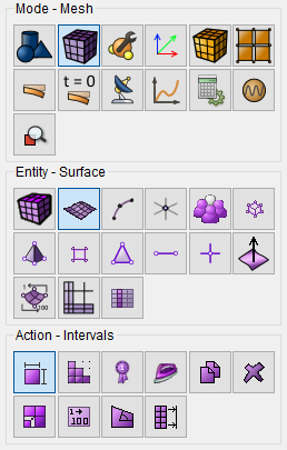
Specify the parameters of mesh refinement:
The way of meshing: Approximate Size;
Select Surfaces: 7;
Approximate Size: 0.125.
Click Apply Size.
2. On the command bar, select the surface mesh module (Mode — Mesh, Entity — Surface, Action — Mesh).
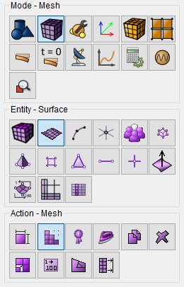
Select meshing scheme:
Select meshing scheme: Polyhedron;
Select Surfaces: 7.
Click Apply Scheme.
Click Mesh.
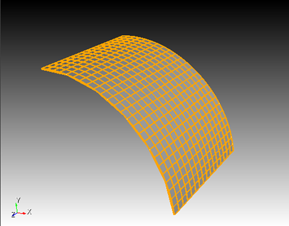
1. Fix the line AB on the conditions of symmetry.
On the command panel, select the boundary conditions module (Mode — Boundary Conditions, Entity — Displacement, Action — Create).
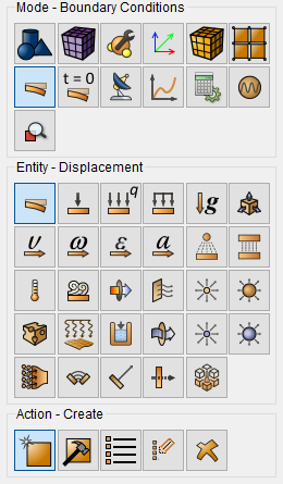
Set the following parameters:
Entity List: Curve;
Entity ID(s): 5 (or click on the top line on a quarter of the shell);
Degrees of Freedom: Х, Y Rotation, Z Rotation.
Click Apply.
2. Fix the line CD of the conditions of symmetry.
On the command panel, select the boundary conditions module (Mode — Boundary Conditions, Entity — Displacement, Action — Create).
Set the following parameters:
Entity List: Curve;
Entity ID(s): 16 (or click on the lower line on a quarter of the shell);
Degrees of Freedom: Y, X-Rotation, Z-Rotation.
Click Apply.
3. Fix the line BC of the conditions of symmetry.
On the command panel, select the boundary conditions module (Mode — Boundary Conditions, Entity — Displacement, Action — Create).
Set the following parameters:
Entity List: Curve;
Entity ID(s): 18;
Degrees of Freedom: Z.
Click Apply.
4. Apply pressure to the entire surface of the shell.
On the command panel, select the boundary conditions module (Mode — Boundary Conditions, Entity — Pressure, Action — Create).
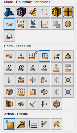
Set the following parameters:
Entity List: Surface;
Entity ID(s): 7;
Value: 1000.
Click Apply.
1. Create the material.
In the command bar, select the module for specifying material properties (Mode — Material, Entity — Materials Management).

In the Materials Management window that opens, in the second column, click on the caption Enter the name of the material and write “Material 1”.
Click the ENTER key.
In the left column, select Elasticity - Isotropic Material. Select with the mouse the characteristic Young's modulus. Hold down the left mouse button and drag the label to Material Properties. Double-click in the Value field next to Young’s modulus and enter the number 2e+11. Similarly, from the Isotropic Material section add the Poisson ratio 0.3.
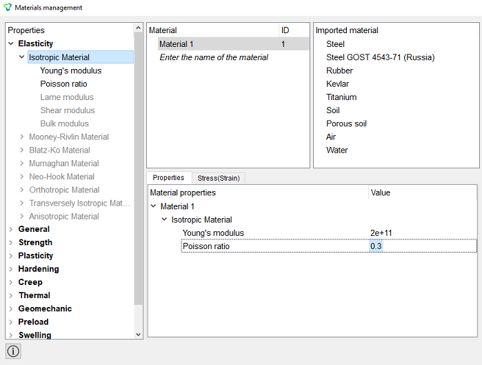
Click Apply.
Close the Materials management window.
2. Create a block of one type of the material.
On the command bar, select the block management module (Mode — Blocks, Entity — Block, Action — Add).

Set the following parameters:
Block ID: 1;
Entity List: Surface;
Entity ID(s): 7 (or by the command all).
Click Apply.
3. Set the block parameters.
On the command bar, select the block management module (Mode - Blocks, Entity - Block, Action - Block properties/parameters).

Set the following parameters:
Block ID(s): 1;
Category: Shell;
Coordinate System: Global Cartesian;
Order: 1.
Set the shell properties by clicking the button  .
.
Set the following parameters:
Material: Material 1;
Thickness: 0.02;
Eccentricity: 0.5.
Click Apply.
Close the window Set Shell Properties.
Click Apply.
1. Set the type of the problem to be solved.
On the command bar, select the calculation settings module (Mode — Calculation Settings, Calculation Settings — Buckling, Buckling — General).
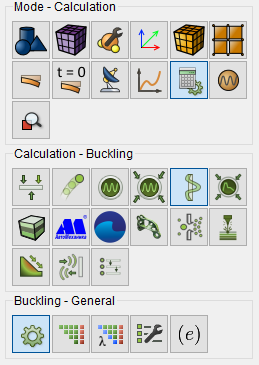
Select:
Dimensions: 3D;
Number of Buckling Modes: 10.
Click Apply.
2. On the command bar, select the calculation settings module (Mode — Calculation Settings, Calculation Settings — Buckling, Buckling — Output Fields).
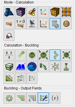
Select:
Results in 3D view (for Beams and Shells).
Click Apply.
Click Start Calculation.
3. In a pop-up window select a folder to save the result and enter the file name.
4. In the case of a successful calculation, the console displays the message: Calculation finished successfully at "date" "time".
1. Compare the obtained results.
The first three critical values are displayed in Command Line.
Compare the obtained results with those in the table:
| № | Theor. value | CAE Fidesys | Error, % |
| 1 | 54.172 | 54.1708 | 0.00 |
| 2 | 270.77 | 270.733 | 0.01 |
| 3 | 631.3 | 631.106 | 0.03 |
2. Open the file with the results. There are three ways to do that.
Click Ctrl+E.
From the main menu, select Calculation. Click Open Results.
Select Results on Command Panel (Mode - Results). Click Open results.

3. In a pop-up Fidesys Viewer window select a filter Warp By Vector.
.png)
4. In a pop-up filter Warp By Vector in the tab Properties, set the following parameters:
Vectors: Mode 1 displacement;
Scale Factor: 0.1.
5. Display Mode 1 displacement.
In Fidesys Viewer window set the following parameters on Toolbar:

Make sure that the first required critical value is displayed in the window Critical value.
6. View results.
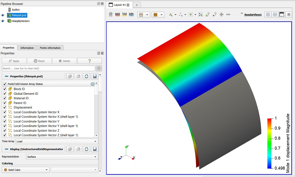
As a result, the deformed body is displayed at the picture. To see the
original model, click .png) near the model in the Model
Tree. The picture below shows the deformed (solid grey filling) and the
original model (with the distribution field Displacements for Mode 1).
near the model in the Model
Tree. The picture below shows the deformed (solid grey filling) and the
original model (with the distribution field Displacements for Mode 1).
7. Select the filter Warp By Vector to do this. Set the following field value in the tab Properties:
Vectors: Mode 2 displacement;
Scale Factor: 0.1.
8. Display Mode 2 displacement.
In Fidesys Viewer window set the following parameters on Toolbar:

Make sure that the second required critical value is displayed in the window Critical value.
9. View results.
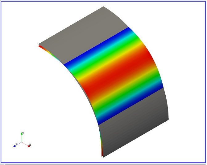
10. Similarly display Displacements for mode 3, make sure that the third required critical value is displayed in the window Critical value.
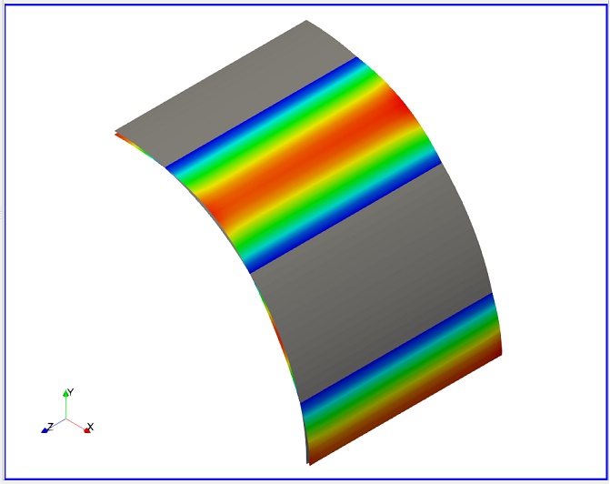
11. Display the 3D-view of the model (shell with thickness).
To do this, click on the name of the source file in the Model Tree. After this click 3D-view button in the default string.
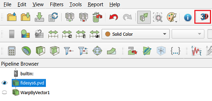
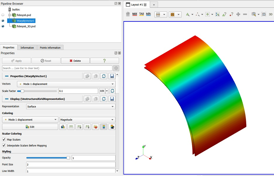
The file* _3D.pvd with a 3D-image of the shell must be opened and you will be able to apply various filters to it and to view its deformed view.
Choose the new file example_3D.pvd in the Model Tree and display Filters Warp by Vector for it with the following fields values:
Vectors: Mode 1 displacement;
Scale Factor: 0.1.
On the Toolbar, set once again the following parameters for the deformed type:

The first buckling mode will be displayed on the screen but the shell will be enveloped with thickness.
.png) To apply
all of the filters’ changes automatically, click Apply changes to parameters
automatically on Command Panel.
To apply
all of the filters’ changes automatically, click Apply changes to parameters
automatically on Command Panel.
12. Download numerical data.
Select File → Save Data in the Main Menu or click Ctrl+S. Enter the file name (*.csv format), leave it by default. Click OK.
The saved file is an ordinary table of numerical data which can be opened in any text editor.
Geometry creating, meshing, setting boundary conditions and materials can be performed using the console interface. Below is a link to the program code that allows you to perform the steps described above manual, you only need to specify the full path and name.