Search the documentation
Enter at least 2 characters
Enter at least 2 characters
 |
CAE Fidesys 9.0 Documentation |
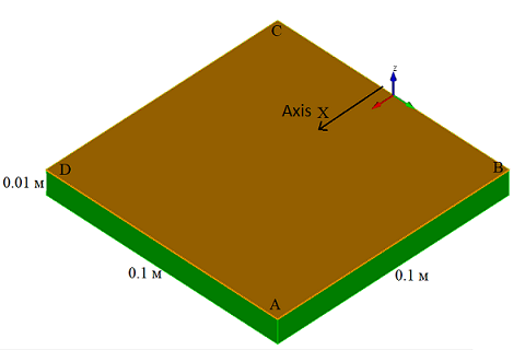
An example of calculating the thermal process during welding is considered (imitation of heating from the welding arc through a normally circular source). The design is a flat plate. From above, a heat flux is set on it according to the formula of a normal-circular heating source.
Normal-circular heat source is given by the formula:
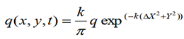
where:
ΔX - move along the OX axis;
k - dispersal factor, м-2;
q - effective power of the welding arc, Watt.
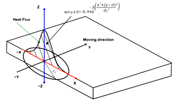
Graphical rendering of a normal-circular source:
1. Create a brick.
On the command bar, select the module for constructing volume geometry (Mode - Geometry, Entity - Volume, Action - Create).
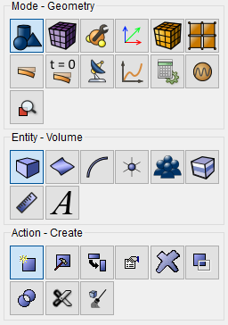
From the list of geometric primitives, select Brick.
Set the following parameters:
X (width): 0.1;
Y (height): 0.1;
Z (depth): 0.01.
Click Apply.
2. Move the entity.
On the command bar, select the module for constructing volume geometry (Mode - Geometry, Entity - Volume, Action - Transform).
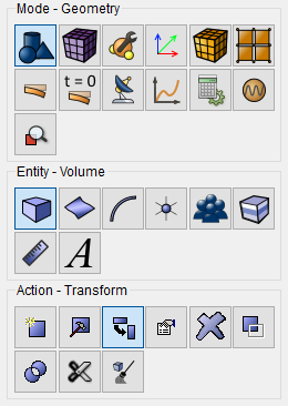
Select Move from the list of possible types of slices.
et the following parameters:
Volumes ID(s): all;
Put a tick: Include Merged;
Select Method: Distance;
Х Distance: 0.05;
Z Distance: -0.005.
Click Apply.
1. On the command bar, select the volume mesh module (Mode - Mesh, Entity - Volume, Action - Intervals).
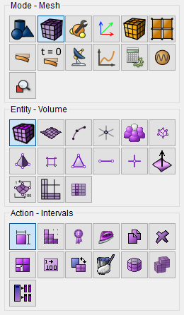
Specify the Approximate Size of the elements:
Select Volumes: all;
Approximate Size: 0.002.
Click Apply Scheme.
Click Mesh.
1. Create the material.
In the command bar, select the module for specifying material properties (Mode - Material, Entity - Materials Management).

In the opened widget Material management in the middle column specify the material name test.
In the property column, open the General list and drag the title Density in the Material properties column.
In the property column, open the Termal list and drag name Specific heat coefficient in the column Properties Material.
In the properties column, open the list Termal, Termal Isotropic and drag title Thermal conductivity coefficient to the Material properties column.
Fill in the properties as follows:
Density: 8000;
Specific heat coefficient: 500;
Thermal conductivity coefficient: 30.
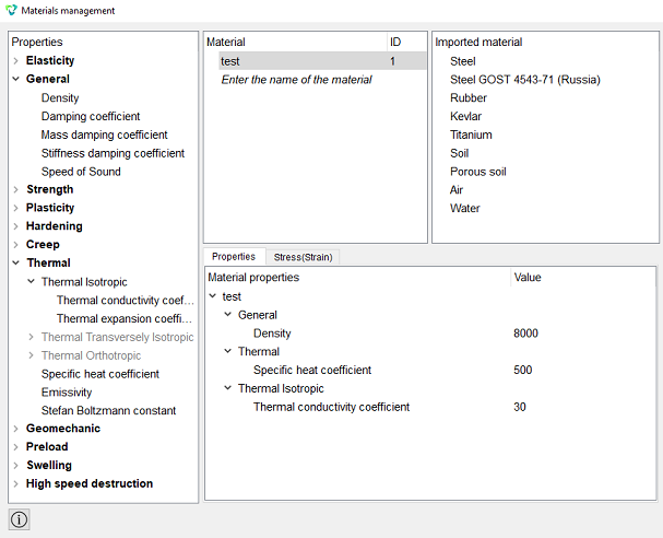
Click Apply.
Close the Materials management window.
2. Create a block.
Select setting the material properties section on Command Panel (Mode - Blocks, Entity - Block, Action - Add).

Set the following parameters:
Block ID: 1;
Entity List: Volume;
Entity ID(s): all.
Click Apply.
3. Set the block parameters.
On the command bar, select the block management module (Mode - Blocks, Entity - Block, Action - Block properties/parameters).

Set the following parameters:
Block ID(s): 1;
Category: Solid;
Material: test;
Coordinate System: Global Cartesian;
Order: 1.
Click Apply.
1. Set the heat flux.
On the command panel, select the boundary conditions module (Mode - Boundary Conditions, Entity - Heatflux, Action - Create).
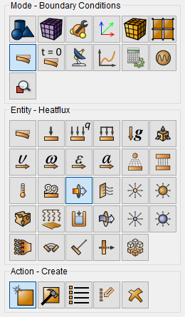
Set the following parameters:
Entity List: Surface;
Entity ID(s): 1;
Surrounding;
Flux: 1.
Click Apply.
1. Set the start temperature
Select on Command Panel (Mode - Initial Conditions, Entity - Temperature, Action - Create).
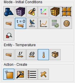
Set the following parameters:
Entity List: Volume;
Entity ID(s): all;
Value: 20.
Click Apply.
On the command panel, select the module for specifying Dependency BC (Mode - BC Dependency).
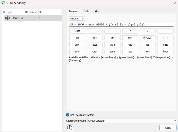
In the BC Dependency window that appears, set the required parameters.
Click Apply.
Close the BC Dependency window.
1. Set the type of problem you want to solve.
On the command panel, select the calculation settings module (Mode - Calculation Settings, Calculation Settings - Transient Analysis, Transient - General).
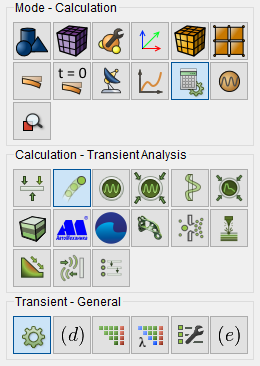
Set the following calculation parameters:
Dimension: 3D;
Method: Full Solution;
Scheme: Implicit;
Max Time: 5;
Steps Count: 50;
Model: uncheck the Elasticity box (it is checked by default);
Model: Heat Transfer.
Click Apply.
2. Specify the temperature in the medium properties.
On the command bar, select the calculation settings module (Mode - Calculation Settings, Calculation Settings - Transient Analysis, Transient - Environment Properties).
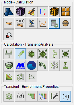
Set the following calculation parameters:
Temperature: 20.
Click Apply.
3. Set the output fields.
On the command bar, select the calculation settings module (Mode - Calculation Settings, Calculation Settings - Transient Analysis, Transient - Output Fields).
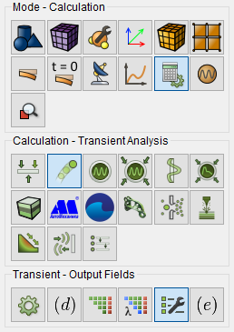
Set the following calculation parameters:
Click Apply.
Click Start Calculation.
4. In the window that appears, select the directory in which the result will be saved, and enter the file name.
5. In the case of a successful calculation, the console displays the message: Calculation finished successfully at "date" "time".
1. Open the file with the results. There are three ways to do that.
Click Ctrl+E.
From the main menu, select Calculation. Click Open Results.
Select Results on Command Panel (Mode - Results). Click Open results.

2. For post-processing analysis, switch to the FidesysViewer window.
3. On the top bar, select the calculation result data to display. From the first from the drop-down list, select Temperature, from the third - Surface.
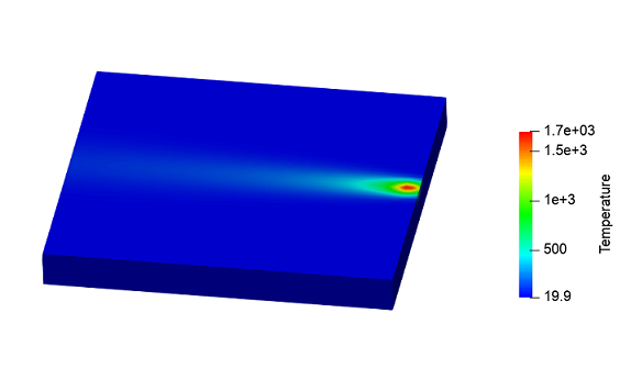
Geometry creating, meshing, setting boundary conditions and materials can be performed using the console interface. Below is a link to the program code that allows you to perform the steps described above manual, you only need to specify the full path and name.